Robot Dynamics

Robotics

Robot Dynamics encompasses the analysis of forces like Coriolis effects, mass distribution, and gravity on a robot, crucial for designing control strategies. This understanding ensures precise and stable movements in various operational scenarios

Robot Dynamics

Here we will simulate the dynamics of the planar robot shown above. We have the dynamics of this robot mentioned in the code.

Now we combine our simulation with the dynamics we have for the specified robot. We will need to get the (𝑥, 𝑦) position of each link to plot the robot. We are using the given simulation parameters and frame rates.

Make a simulation where $\normalsize \tau = [0, 0]^{𝑇}$ and the robot has no friction.
Make a simulation where $\normalsize \tau = [0, 0]^{𝑇}$ and the robot has viscous friction 𝐵 = 𝐼.
Make a simulation where $\normalsize \tau = [20, 5]^{𝑇}$ and the robot has viscous friction 𝐵 = 𝐼.

We can play with the parameters (such as mass, inertia, friction, and 𝜏), and see how these parameters affect the simulation. We can see the implementations below for the simulation codes I am responsible for.

Environment 1: Make a simulation where $\normalsize \tau = [0, 0]^{𝑇}$ and the robot has no friction.

Implementations

Python

Code

import numpy as np
import matplotlib
matplotlib.use('Agg')  # Set the backend to a non-interactive backend
import matplotlib.pyplot as plt
import matplotlib.animation as animation
from matplotlib.animation import PillowWriter
from scipy.spatial.transform import Rotation as R

def expm(A):
    return np.linalg.matrix_power(np.eye(A.shape[0]) + A / 16, 16)

def bracket_s(s):
    return np.array([[0, -s[2], s[1], s[3]], [s[2], 0, -s[0], s[4]], [-s[1], s[0], 0, s[5]], [0, 0, 0, 0]])

def fk(M, S, theta):
    T = np.eye(4)
    for i in range(len(theta)):
        T = np.dot(T, expm(bracket_s(S[:, i]) * theta[i]))
    return np.dot(T, M)

# System parameters
L1 = 1
L2 = 1
m1 = 1
m2 = 1
I1 = 0.1
I2 = 0.1
g = 9.81
tau = np.array([0, 0])  # Case 1

# Initial conditions
theta = np.array([0.0, 0.0])
thetadot = np.array([0.0, 0.0])
thetadotdot = np.array([0.0, 0.0])

omega = np.array([0, 0, 1])
q1 = np.array([0, 0, 0])
q2 = np.array([L1, 0, 0])
q3 = np.array([L1 + L2, 0, 0])

S1 = np.hstack((omega, -np.cross(omega, q1)))
S2 = np.hstack((omega, -np.cross(omega, q2)))
S_eq1 = np.column_stack((S1, np.zeros(6)))
S_eq2 = np.column_stack((S1, S2))

M1 = np.vstack((np.hstack((np.eye(3), q2[:, None])), [0, 0, 0, 1]))
M2 = np.vstack((np.hstack((np.eye(3), np.array([[L1 + L2, 0, 0]]).T)), [0, 0, 0, 1]))

# Plot setup
max_reach = L1 + L2
fig, ax = plt.subplots()
ax.set_xlim(-3, 3)
ax.set_ylim(-3, 3)
ax.grid()

# Animation setup
frames = 1000
deltaT = 0.01
lines, = ax.plot([], [], 'o-', color=[1, 0.5, 0], linewidth=4)


def animate(idx):
    global theta, thetadot, thetadotdot
    p0 = np.array([0,0])
    T1 = fk(M1, S_eq2[:, 0:1], theta[0:1])
    p1 = T1[0:2, 3]
    T2 = fk(M2, S_eq2, theta)
    p2 = T2[0:2, 3]
    P = np.column_stack((p0, p1, p2))

    lines.set_data(P[0, :], P[1, :])

    thetadot += deltaT * thetadotdot
    theta += deltaT * thetadot

    # Dynamics and integration
    Mass_Matrix = np.array([
        [I1 + I2 + L1**2*m1 + L1**2*m2 + L2**2*m2 + 2*L1*L2*m2*np.cos(theta[1]), m2*L2**2 + L1*m2*np.cos(theta[1])*L2 + I2],
        [m2*L2**2 + L1*m2*np.cos(theta[1])*L2 + I2, m2*L2**2 + I2]
    ])

    Coriolis_Matrix = np.array([
        [-L1*L2*m2*thetadot[1]*np.sin(theta[1]), -L1*L2*m2*np.sin(theta[1])*(thetadot[0] + thetadot[1])],
        [L1*L2*m2*thetadot[0]*np.sin(theta[1]), 0]
    ])

    gravity_vector = np.array([
        g*(m1 + m2)*L1*np.cos(theta[0]) + g*m2*L2*np.cos(np.sum(theta)),
        g*m2*L2*np.cos(np.sum(theta))
    ])

    B = np.array([[0, 0], [0, 0]])  # Case 1

    thetadotdot = np.linalg.inv(Mass_Matrix) @ (tau - Coriolis_Matrix @ thetadot - B @ thetadot - gravity_vector)
 

    return lines,

ani = animation.FuncAnimation(fig, animate, frames=frames, interval=deltaT*1000, blit=False)

# Save as GIF
ani.save('Pendulum_Python_1.gif', writer=PillowWriter(fps=33))

MATLAB

Code


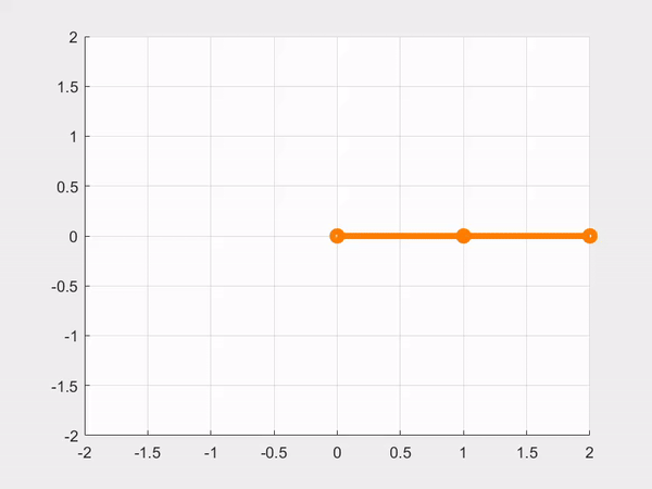
close all
clear
clc


% create figure
figure
axis([-2, 2, -2, 2])
grid on
hold on

% save as a video file
v = VideoWriter('Pendulum_Case_1.mp4', 'MPEG-4');
v.FrameRate = 100;
open(v);

% pick your system parameters
L1 = 1;
L2 = 1;
m1 = 1;
m2 = 1;
I1 = 0.1;
I2 = 0.1;
g = 9.81;
tau = [0;0]; % Case 1

% Initial conditions
theta = [0;0]; % joint position
thetadot = [0;0]; % joint velocity
thetadotdot = [0;0]; % joint acceleration

masses = [m1,m2];
omega = [0;0;1];

Inertia_1 = [0 0 0;0 0 0;0 0 I1];
Inertia_2 = [0 0 0;0 0 0;0 0 I2];
q1 = [0;0;0]; % Position of Joint 1
q2 = [L1;0;0]; % Position of Joint 2
q3 = [L1+L2;0;0]; % end effector position

S1 = [omega; -cross(omega,q1)];
S2 = [omega;-cross(omega,q2)];
S_eq1 = [S1,[0;0;0;0;0;0]];
S_eq2 = [S1, S2]; 

M1 = [eye(3),q2; 0 0 0 1];
M2 = [eye(3), [L1+L2;0;0]; 0 0 0 1];

gravity_vector = (zeros(length(theta),1));
Coriolis_Matrix = (zeros(2,2));
Mass_Matrix = [I1 + I2 + L1^2*m1 + L1^2*m2 + L2^2*m2 + 2*L1*L2*m2*cos(theta(2)), m2*L2^2 + L1*m2*cos(theta(2))*L2 + I2; m2*L2^2 + L1*m2*cos(theta(2))*L2 + I2, m2*L2^2 + I2];
    

for idx = 1:1000

    % plot the robot
    % 1. get the position of each link
    p0 = [0; 0];
    T1 = fk(M1,S_eq2(:,1:1),theta(1:1,:));
    p1 = T1(1:2,4); % position of link 1 (location of joint 2)
    T2 = fk(M2,S_eq2,theta);
    p2 = T2(1:2,4); % position of link 2 (the end-effector)
    P = [p0, p1, p2];
    % 2. draw the robot and save the frame
    cla;
    plot(P(1,:), P(2,:), 'o-', 'color',[1, 0.5, 0],'linewidth',4);
    drawnow;
    frame = getframe(gcf);
    writeVideo(v,frame);

    % integrate to update velocity and position
    % your code here
    deltaT = 0.01;
    thetadot = thetadot + deltaT * thetadotdot;
    theta = theta + deltaT * thetadot;

    Mass_Matrix =[I1 + I2 + L1^2*m1 + L1^2*m2 + L2^2*m2 + 2*L1*L2*m2*cos(theta(2)), m2*L2^2 + L1*m2*cos(theta(2))*L2 + I2; m2*L2^2 + L1*m2*cos(theta(2))*L2 + I2, m2*L2^2 + I2];
    
    Coriolis_Matrix = [-L1*L2*m2*thetadot(2)*sin(theta(2)),  -L1*L2*m2*sin(theta(2))*(thetadot(1) + thetadot(2));L1*L2*m2*thetadot(1)*sin(theta(2)), 0] ;
    
    gravity_vector = [(g*(m1+m2)*L1*cos(theta(1))) + g*m2*L2*cos(theta(1) + theta(2)); g*m2*L2*cos(theta(1) + theta(2))];
    
    B = [[0 0]
        [0 0]]; % Case 1

    thetadotdot = (inv(Mass_Matrix)) * (tau - Coriolis_Matrix * thetadot -B*thetadot - gravity_vector);

end

close(v);
close all

Result:

Animated GIF

Environment 2: Make a simulation where $\normalsize \tau = [0, 0]^𝑇$ and the robot has viscous friction $\normalsize 𝐵 = 𝐼$.

Implementations

Python

Code

import numpy as np
import matplotlib
matplotlib.use('Agg')  # Set the backend to a non-interactive backend
import matplotlib.pyplot as plt
import matplotlib.animation as animation
from matplotlib.animation import PillowWriter
from scipy.spatial.transform import Rotation as R

def expm(A):
    return np.linalg.matrix_power(np.eye(A.shape[0]) + A / 16, 16)

def bracket_s(s):
    return np.array([[0, -s[2], s[1], s[3]], [s[2], 0, -s[0], s[4]], [-s[1], s[0], 0, s[5]], [0, 0, 0, 0]])

def fk(M, S, theta):
    T = np.eye(4)
    for i in range(len(theta)):
        T = np.dot(T, expm(bracket_s(S[:, i]) * theta[i]))
    return np.dot(T, M)

# System parameters
L1 = 1
L2 = 1
m1 = 1
m2 = 1
I1 = 0.1
I2 = 0.1
g = 9.81
tau = np.array([0, 0])  # Case 2

# Initial conditions
theta = np.array([0.0, 0.0])
thetadot = np.array([0.0, 0.0])
thetadotdot = np.array([0.0, 0.0])

omega = np.array([0, 0, 1])
q1 = np.array([0, 0, 0])
q2 = np.array([L1, 0, 0])
q3 = np.array([L1 + L2, 0, 0])

S1 = np.hstack((omega, -np.cross(omega, q1)))
S2 = np.hstack((omega, -np.cross(omega, q2)))
S_eq1 = np.column_stack((S1, np.zeros(6)))
S_eq2 = np.column_stack((S1, S2))

M1 = np.vstack((np.hstack((np.eye(3), q2[:, None])), [0, 0, 0, 1]))
M2 = np.vstack((np.hstack((np.eye(3), np.array([[L1 + L2, 0, 0]]).T)), [0, 0, 0, 1]))

# Plot setup
max_reach = L1 + L2
fig, ax = plt.subplots()
ax.set_xlim(-3, 3)
ax.set_ylim(-3, 3)
ax.grid()

# Animation setup
frames = 1000
deltaT = 0.01
lines, = ax.plot([], [], 'o-', color=[1, 0.5, 0], linewidth=4)


def animate(idx):
    global theta, thetadot, thetadotdot
    p0 = np.array([0,0])
    T1 = fk(M1, S_eq2[:, 0:1], theta[0:1])
    p1 = T1[0:2, 3]
    T2 = fk(M2, S_eq2, theta)
    p2 = T2[0:2, 3]
    P = np.column_stack((p0, p1, p2))

    lines.set_data(P[0, :], P[1, :])

    thetadot += deltaT * thetadotdot
    theta += deltaT * thetadot

    # Dynamics and integration
    Mass_Matrix = np.array([
        [I1 + I2 + L1**2*m1 + L1**2*m2 + L2**2*m2 + 2*L1*L2*m2*np.cos(theta[1]), m2*L2**2 + L1*m2*np.cos(theta[1])*L2 + I2],
        [m2*L2**2 + L1*m2*np.cos(theta[1])*L2 + I2, m2*L2**2 + I2]
    ])

    Coriolis_Matrix = np.array([
        [-L1*L2*m2*thetadot[1]*np.sin(theta[1]), -L1*L2*m2*np.sin(theta[1])*(thetadot[0] + thetadot[1])],
        [L1*L2*m2*thetadot[0]*np.sin(theta[1]), 0]
    ])

    gravity_vector = np.array([
        g*(m1 + m2)*L1*np.cos(theta[0]) + g*m2*L2*np.cos(np.sum(theta)),
        g*m2*L2*np.cos(np.sum(theta))
    ])

    B = np.array([[1, 0], [0, 1]])  # Case 2

    thetadotdot = np.linalg.inv(Mass_Matrix) @ (tau - Coriolis_Matrix @ thetadot - B @ thetadot - gravity_vector)
 

    return lines,

ani = animation.FuncAnimation(fig, animate, frames=frames, interval=deltaT*1000, blit=False)

# Save as GIF
ani.save('Pendulum_Python_2.gif', writer=PillowWriter(fps=33))

MATLAB

Code


close all
clear
clc

% create figure
figure
axis([-2, 2, -2, 2])
grid on
hold on

% save as a video file
v = VideoWriter('Pendulum_Case_2.mp4', 'MPEG-4');
v.FrameRate = 100;
open(v);

% pick your system parameters
L1 = 1;
L2 = 1;
m1 = 1;
m2 = 1;
I1 = 0.1;
I2 = 0.1;
g = 9.81;
tau = [0;0]; % Case 2

% Initial conditions
theta = [0;0]; % joint position
thetadot = [0;0]; % joint velocity
thetadotdot = [0;0]; % joint acceleration

masses = [m1,m2];
omega = [0;0;1];

Inertia_1 = [0 0 0;0 0 0;0 0 I1];
Inertia_2 = [0 0 0;0 0 0;0 0 I2];
q1 = [0;0;0]; % Position of Joint 1
q2 = [L1;0;0]; % Position of Joint 2
q3 = [L1+L2;0;0]; % end effector position

S1 = [omega; -cross(omega,q1)];
S2 = [omega;-cross(omega,q2)];
S_eq1 = [S1,[0;0;0;0;0;0]];
S_eq2 = [S1, S2]; 

M1 = [eye(3),q2; 0 0 0 1];
M2 = [eye(3), [L1+L2;0;0]; 0 0 0 1];

gravity_vector = (zeros(length(theta),1));
Coriolis_Matrix = (zeros(2,2));
Mass_Matrix = [I1 + I2 + L1^2*m1 + L1^2*m2 + L2^2*m2 + 2*L1*L2*m2*cos(theta(2)), m2*L2^2 + L1*m2*cos(theta(2))*L2 + I2; m2*L2^2 + L1*m2*cos(theta(2))*L2 + I2, m2*L2^2 + I2];
    

for idx = 1:1000

    % plot the robot
    % 1. get the position of each link
    p0 = [0; 0];
    T1 = fk(M1,S_eq2(:,1:1),theta(1:1,:));
    p1 = T1(1:2,4); % position of link 1 (location of joint 2)
    T2 = fk(M2,S_eq2,theta);
    p2 = T2(1:2,4); % position of link 2 (the end-effector)
    P = [p0, p1, p2];
    % 2. draw the robot and save the frame
    cla;
    plot(P(1,:), P(2,:), 'o-', 'color',[1, 0.5, 0],'linewidth',4);
    drawnow;
    frame = getframe(gcf);
    writeVideo(v,frame);

    % integrate to update velocity and position
    % your code here
    deltaT = 0.01;
    thetadot = thetadot + deltaT * thetadotdot;
    theta = theta + deltaT * thetadot;

    Mass_Matrix =[I1 + I2 + L1^2*m1 + L1^2*m2 + L2^2*m2 + 2*L1*L2*m2*cos(theta(2)), m2*L2^2 + L1*m2*cos(theta(2))*L2 + I2; m2*L2^2 + L1*m2*cos(theta(2))*L2 + I2, m2*L2^2 + I2];
    
    Coriolis_Matrix = [-L1*L2*m2*thetadot(2)*sin(theta(2)),  -L1*L2*m2*sin(theta(2))*(thetadot(1) + thetadot(2));L1*L2*m2*thetadot(1)*sin(theta(2)), 0] ;
    
    gravity_vector = [(g*(m1+m2)*L1*cos(theta(1))) + g*m2*L2*cos(theta(1) + theta(2)); g*m2*L2*cos(theta(1) + theta(2))];
    
    B = eye(2); % Case 2

    thetadotdot = (inv(Mass_Matrix)) * (tau - Coriolis_Matrix * thetadot -B*thetadot - gravity_vector);

end

close(v);
close all

Result:

Animated GIF

Environment 3: Make a simulation where $\normalsize \tau = [20, 5]^𝑇$ and the robot has viscous friction $\normalsize 𝐵 = 𝐼$.

Implementations

Python

Code

import numpy as np
import matplotlib
matplotlib.use('Agg')  # Set the backend to a non-interactive backend
import matplotlib.pyplot as plt
import matplotlib.animation as animation
from matplotlib.animation import PillowWriter
from scipy.spatial.transform import Rotation as R

def expm(A):
    return np.linalg.matrix_power(np.eye(A.shape[0]) + A / 16, 16)

def bracket_s(s):
    return np.array([[0, -s[2], s[1], s[3]], [s[2], 0, -s[0], s[4]], [-s[1], s[0], 0, s[5]], [0, 0, 0, 0]])

def fk(M, S, theta):
    T = np.eye(4)
    for i in range(len(theta)):
        T = np.dot(T, expm(bracket_s(S[:, i]) * theta[i]))
    return np.dot(T, M)

# System parameters
L1 = 1
L2 = 1
m1 = 1
m2 = 1
I1 = 0.1
I2 = 0.1
g = 9.81
tau = np.array([20, 5])  # Case 3

# Initial conditions
theta = np.array([0.0, 0.0])
thetadot = np.array([0.0, 0.0])
thetadotdot = np.array([0.0, 0.0])

omega = np.array([0, 0, 1])
q1 = np.array([0, 0, 0])
q2 = np.array([L1, 0, 0])
q3 = np.array([L1 + L2, 0, 0])

S1 = np.hstack((omega, -np.cross(omega, q1)))
S2 = np.hstack((omega, -np.cross(omega, q2)))
S_eq1 = np.column_stack((S1, np.zeros(6)))
S_eq2 = np.column_stack((S1, S2))

M1 = np.vstack((np.hstack((np.eye(3), q2[:, None])), [0, 0, 0, 1]))
M2 = np.vstack((np.hstack((np.eye(3), np.array([[L1 + L2, 0, 0]]).T)), [0, 0, 0, 1]))

# Plot setup
max_reach = L1 + L2
fig, ax = plt.subplots()
ax.set_xlim(-3, 3)
ax.set_ylim(-3, 3)
ax.grid()

# Animation setup
frames = 1000
deltaT = 0.01
lines, = ax.plot([], [], 'o-', color=[1, 0.5, 0], linewidth=4)


def animate(idx):
    global theta, thetadot, thetadotdot
    p0 = np.array([0,0])
    T1 = fk(M1, S_eq2[:, 0:1], theta[0:1])
    p1 = T1[0:2, 3]
    T2 = fk(M2, S_eq2, theta)
    p2 = T2[0:2, 3]
    P = np.column_stack((p0, p1, p2))

    lines.set_data(P[0, :], P[1, :])

    thetadot += deltaT * thetadotdot
    theta += deltaT * thetadot

    # Dynamics and integration
    Mass_Matrix = np.array([
        [I1 + I2 + L1**2*m1 + L1**2*m2 + L2**2*m2 + 2*L1*L2*m2*np.cos(theta[1]), m2*L2**2 + L1*m2*np.cos(theta[1])*L2 + I2],
        [m2*L2**2 + L1*m2*np.cos(theta[1])*L2 + I2, m2*L2**2 + I2]
    ])

    Coriolis_Matrix = np.array([
        [-L1*L2*m2*thetadot[1]*np.sin(theta[1]), -L1*L2*m2*np.sin(theta[1])*(thetadot[0] + thetadot[1])],
        [L1*L2*m2*thetadot[0]*np.sin(theta[1]), 0]
    ])

    gravity_vector = np.array([
        g*(m1 + m2)*L1*np.cos(theta[0]) + g*m2*L2*np.cos(np.sum(theta)),
        g*m2*L2*np.cos(np.sum(theta))
    ])

    B = np.array([[1, 0], [0, 1]])  # Case 3

    thetadotdot = np.linalg.inv(Mass_Matrix) @ (tau - Coriolis_Matrix @ thetadot - B @ thetadot - gravity_vector)
 

    return lines,

ani = animation.FuncAnimation(fig, animate, frames=frames, interval=deltaT*1000, blit=False)

# Save as GIF
ani.save('Pendulum_Python_3.gif', writer=PillowWriter(fps=33))

MATLAB

Code


close all
clear
clc


% create figure
figure
axis([-2, 2, -2, 2])
grid on
hold on

% save as a video file
v = VideoWriter('Pendulum_Python_3.mp4', 'MPEG-4');
v.FrameRate = 100;
open(v);

% pick your system parameters
L1 = 1;
L2 = 1;
m1 = 1;
m2 = 1;
I1 = 0.1;
I2 = 0.1;
g = 9.81;
tau = [20;5]; % Case 3

% Initial conditions
theta = [0;0]; % joint position
thetadot = [0;0]; % joint velocity
thetadotdot = [0;0]; % joint acceleration

masses = [m1,m2];
omega = [0;0;1];

Inertia_1 = [0 0 0;0 0 0;0 0 I1];
Inertia_2 = [0 0 0;0 0 0;0 0 I2];
q1 = [0;0;0]; % Position of Joint 1
q2 = [L1;0;0]; % Position of Joint 2
q3 = [L1+L2;0;0]; % end effector position

S1 = [omega; -cross(omega,q1)];
S2 = [omega;-cross(omega,q2)];
S_eq1 = [S1,[0;0;0;0;0;0]];
S_eq2 = [S1, S2]; 

M1 = [eye(3),q2; 0 0 0 1];
M2 = [eye(3), [L1+L2;0;0]; 0 0 0 1];

gravity_vector = (zeros(length(theta),1));
Coriolis_Matrix = (zeros(2,2));
Mass_Matrix = [I1 + I2 + L1^2*m1 + L1^2*m2 + L2^2*m2 + 2*L1*L2*m2*cos(theta(2)), m2*L2^2 + L1*m2*cos(theta(2))*L2 + I2; m2*L2^2 + L1*m2*cos(theta(2))*L2 + I2, m2*L2^2 + I2];
    

for idx = 1:1000

    % plot the robot
    % 1. get the position of each link
    p0 = [0; 0];
    T1 = fk(M1,S_eq2(:,1:1),theta(1:1,:));
    p1 = T1(1:2,4); % position of link 1 (location of joint 2)
    T2 = fk(M2,S_eq2,theta);
    p2 = T2(1:2,4); % position of link 2 (the end-effector)
    P = [p0, p1, p2];
    % 2. draw the robot and save the frame
    cla;
    plot(P(1,:), P(2,:), 'o-', 'color',[1, 0.5, 0],'linewidth',4);
    drawnow;
    frame = getframe(gcf);
    writeVideo(v,frame);

    % integrate to update velocity and position
    % your code here
    deltaT = 0.01;
    thetadot = thetadot + deltaT * thetadotdot;
    theta = theta + deltaT * thetadot;

    Mass_Matrix =[I1 + I2 + L1^2*m1 + L1^2*m2 + L2^2*m2 + 2*L1*L2*m2*cos(theta(2)), m2*L2^2 + L1*m2*cos(theta(2))*L2 + I2; m2*L2^2 + L1*m2*cos(theta(2))*L2 + I2, m2*L2^2 + I2];
    
    Coriolis_Matrix = [-L1*L2*m2*thetadot(2)*sin(theta(2)),  -L1*L2*m2*sin(theta(2))*(thetadot(1) + thetadot(2));L1*L2*m2*thetadot(1)*sin(theta(2)), 0] ;
    
    gravity_vector = [(g*(m1+m2)*L1*cos(theta(1))) + g*m2*L2*cos(theta(1) + theta(2)); g*m2*L2*cos(theta(1) + theta(2))];
    
    B = eye(2); % Case 3

    thetadotdot = (inv(Mass_Matrix)) * (tau - Coriolis_Matrix * thetadot -B*thetadot - gravity_vector);

end

close(v);
close all

Result:

Animated GIF

--- title: "Robot Dynamics" description: "Robot Dynamics encompasses the analysis of forces like Coriolis effects, mass distribution, and gravity on a robot, crucial for designing control strategies. This understanding ensures precise and stable movements in various operational scenarios" categories: [Robotics] image: Dynamics_Pendulum_Cover_GIF.gif format: html: code-fold: show code-overflow: wrap code-tools: true --- ## Robot Dynamics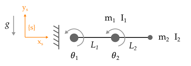 ![](Images/Pendulum_Simulation_Problem.png){fig-align="center" width="50%"} Here we will simulate the dynamics of the planar robot shown above. We have the dynamics of this robot mentioned in the code. Now we combine our simulation with the dynamics we have for the specified robot. We will need to get the (𝑥, 𝑦) position of each link to plot the robot. We are using the given simulation parameters and frame rates. - Make a simulation where $\normalsize \tau = [0, 0]^{𝑇}$ and the robot has no friction. - Make a simulation where $\normalsize \tau = [0, 0]^{𝑇}$ and the robot has viscous friction 𝐵 = 𝐼. - Make a simulation where $\normalsize \tau = [20, 5]^{𝑇}$ and the robot has viscous friction 𝐵 = 𝐼. We can play with the parameters (such as mass, inertia, friction, and 𝜏), and see how these parameters affect the simulation. We can see the implementations below for the simulation codes I am responsible for. - **Environment 1:** Make a simulation where $\normalsize \tau = [0, 0]^{𝑇}$ and the robot has no friction. ### Implementations #### Python ```{python} import numpy as np import matplotlib matplotlib.use('Agg') # Set the backend to a non-interactive backend import matplotlib.pyplot as plt import matplotlib.animation as animation from matplotlib.animation import PillowWriter from scipy.spatial.transform import Rotation as R def expm(A): return np.linalg.matrix_power(np.eye(A.shape[0]) + A / 16, 16) def bracket_s(s): return np.array([[0, -s[2], s[1], s[3]], [s[2], 0, -s[0], s[4]], [-s[1], s[0], 0, s[5]], [0, 0, 0, 0]]) def fk(M, S, theta): T = np.eye(4) for i in range(len(theta)): T = np.dot(T, expm(bracket_s(S[:, i]) * theta[i])) return np.dot(T, M) # System parameters L1 = 1 L2 = 1 m1 = 1 m2 = 1 I1 = 0.1 I2 = 0.1 g = 9.81 tau = np.array([0, 0]) # Case 1 # Initial conditions theta = np.array([0.0, 0.0]) thetadot = np.array([0.0, 0.0]) thetadotdot = np.array([0.0, 0.0]) omega = np.array([0, 0, 1]) q1 = np.array([0, 0, 0]) q2 = np.array([L1, 0, 0]) q3 = np.array([L1 + L2, 0, 0]) S1 = np.hstack((omega, -np.cross(omega, q1))) S2 = np.hstack((omega, -np.cross(omega, q2))) S_eq1 = np.column_stack((S1, np.zeros(6))) S_eq2 = np.column_stack((S1, S2)) M1 = np.vstack((np.hstack((np.eye(3), q2[:, None])), [0, 0, 0, 1])) M2 = np.vstack((np.hstack((np.eye(3), np.array([[L1 + L2, 0, 0]]).T)), [0, 0, 0, 1])) # Plot setup max_reach = L1 + L2 fig, ax = plt.subplots() ax.set_xlim(-3, 3) ax.set_ylim(-3, 3) ax.grid() # Animation setup frames = 1000 deltaT = 0.01 lines, = ax.plot([], [], 'o-', color=[1, 0.5, 0], linewidth=4) def animate(idx): global theta, thetadot, thetadotdot p0 = np.array([0,0]) T1 = fk(M1, S_eq2[:, 0:1], theta[0:1]) p1 = T1[0:2, 3] T2 = fk(M2, S_eq2, theta) p2 = T2[0:2, 3] P = np.column_stack((p0, p1, p2)) lines.set_data(P[0, :], P[1, :]) thetadot += deltaT * thetadotdot theta += deltaT * thetadot # Dynamics and integration Mass_Matrix = np.array([ [I1 + I2 + L1**2*m1 + L1**2*m2 + L2**2*m2 + 2*L1*L2*m2*np.cos(theta[1]), m2*L2**2 + L1*m2*np.cos(theta[1])*L2 + I2], [m2*L2**2 + L1*m2*np.cos(theta[1])*L2 + I2, m2*L2**2 + I2] ]) Coriolis_Matrix = np.array([ [-L1*L2*m2*thetadot[1]*np.sin(theta[1]), -L1*L2*m2*np.sin(theta[1])*(thetadot[0] + thetadot[1])], [L1*L2*m2*thetadot[0]*np.sin(theta[1]), 0] ]) gravity_vector = np.array([ g*(m1 + m2)*L1*np.cos(theta[0]) + g*m2*L2*np.cos(np.sum(theta)), g*m2*L2*np.cos(np.sum(theta)) ]) B = np.array([[0, 0], [0, 0]]) # Case 1 thetadotdot = np.linalg.inv(Mass_Matrix) @ (tau - Coriolis_Matrix @ thetadot - B @ thetadot - gravity_vector) return lines, ani = animation.FuncAnimation(fig, animate, frames=frames, interval=deltaT*1000, blit=False) # Save as GIF ani.save('Pendulum_Python_1.gif', writer=PillowWriter(fps=33)) ``` #### MATLAB <details> <summary>Code</summary> ``` matlab close all clear clc % create figure figure axis([-2, 2, -2, 2]) grid on hold on % save as a video file v = VideoWriter('Pendulum_Case_1.mp4', 'MPEG-4'); v.FrameRate = 100; open(v); % pick your system parameters L1 = 1; L2 = 1; m1 = 1; m2 = 1; I1 = 0.1; I2 = 0.1; g = 9.81; tau = [0;0]; % Case 1 % Initial conditions theta = [0;0]; % joint position thetadot = [0;0]; % joint velocity thetadotdot = [0;0]; % joint acceleration masses = [m1,m2]; omega = [0;0;1]; Inertia_1 = [0 0 0;0 0 0;0 0 I1]; Inertia_2 = [0 0 0;0 0 0;0 0 I2]; q1 = [0;0;0]; % Position of Joint 1 q2 = [L1;0;0]; % Position of Joint 2 q3 = [L1+L2;0;0]; % end effector position S1 = [omega; -cross(omega,q1)]; S2 = [omega;-cross(omega,q2)]; S_eq1 = [S1,[0;0;0;0;0;0]]; S_eq2 = [S1, S2]; M1 = [eye(3),q2; 0 0 0 1]; M2 = [eye(3), [L1+L2;0;0]; 0 0 0 1]; gravity_vector = (zeros(length(theta),1)); Coriolis_Matrix = (zeros(2,2)); Mass_Matrix = [I1 + I2 + L1^2*m1 + L1^2*m2 + L2^2*m2 + 2*L1*L2*m2*cos(theta(2)), m2*L2^2 + L1*m2*cos(theta(2))*L2 + I2; m2*L2^2 + L1*m2*cos(theta(2))*L2 + I2, m2*L2^2 + I2]; for idx = 1:1000 % plot the robot % 1. get the position of each link p0 = [0; 0]; T1 = fk(M1,S_eq2(:,1:1),theta(1:1,:)); p1 = T1(1:2,4); % position of link 1 (location of joint 2) T2 = fk(M2,S_eq2,theta); p2 = T2(1:2,4); % position of link 2 (the end-effector) P = [p0, p1, p2]; % 2. draw the robot and save the frame cla; plot(P(1,:), P(2,:), 'o-', 'color',[1, 0.5, 0],'linewidth',4); drawnow; frame = getframe(gcf); writeVideo(v,frame); % integrate to update velocity and position % your code here deltaT = 0.01; thetadot = thetadot + deltaT * thetadotdot; theta = theta + deltaT * thetadot; Mass_Matrix =[I1 + I2 + L1^2*m1 + L1^2*m2 + L2^2*m2 + 2*L1*L2*m2*cos(theta(2)), m2*L2^2 + L1*m2*cos(theta(2))*L2 + I2; m2*L2^2 + L1*m2*cos(theta(2))*L2 + I2, m2*L2^2 + I2]; Coriolis_Matrix = [-L1*L2*m2*thetadot(2)*sin(theta(2)), -L1*L2*m2*sin(theta(2))*(thetadot(1) + thetadot(2));L1*L2*m2*thetadot(1)*sin(theta(2)), 0] ; gravity_vector = [(g*(m1+m2)*L1*cos(theta(1))) + g*m2*L2*cos(theta(1) + theta(2)); g*m2*L2*cos(theta(1) + theta(2))]; B = [[0 0] [0 0]]; % Case 1 thetadotdot = (inv(Mass_Matrix)) * (tau - Coriolis_Matrix * thetadot -B*thetadot - gravity_vector); end close(v); close all ``` </details> #### Result: <img src="Pendulum_Case_1.gif" alt="Animated GIF" width="50%" height="100%"/> - **Environment 2:** Make a simulation where $\normalsize \tau = [0, 0]^𝑇$ and the robot has viscous friction $\normalsize 𝐵 = 𝐼$. ### Implementations #### Python ```{python} import numpy as np import matplotlib matplotlib.use('Agg') # Set the backend to a non-interactive backend import matplotlib.pyplot as plt import matplotlib.animation as animation from matplotlib.animation import PillowWriter from scipy.spatial.transform import Rotation as R def expm(A): return np.linalg.matrix_power(np.eye(A.shape[0]) + A / 16, 16) def bracket_s(s): return np.array([[0, -s[2], s[1], s[3]], [s[2], 0, -s[0], s[4]], [-s[1], s[0], 0, s[5]], [0, 0, 0, 0]]) def fk(M, S, theta): T = np.eye(4) for i in range(len(theta)): T = np.dot(T, expm(bracket_s(S[:, i]) * theta[i])) return np.dot(T, M) # System parameters L1 = 1 L2 = 1 m1 = 1 m2 = 1 I1 = 0.1 I2 = 0.1 g = 9.81 tau = np.array([0, 0]) # Case 2 # Initial conditions theta = np.array([0.0, 0.0]) thetadot = np.array([0.0, 0.0]) thetadotdot = np.array([0.0, 0.0]) omega = np.array([0, 0, 1]) q1 = np.array([0, 0, 0]) q2 = np.array([L1, 0, 0]) q3 = np.array([L1 + L2, 0, 0]) S1 = np.hstack((omega, -np.cross(omega, q1))) S2 = np.hstack((omega, -np.cross(omega, q2))) S_eq1 = np.column_stack((S1, np.zeros(6))) S_eq2 = np.column_stack((S1, S2)) M1 = np.vstack((np.hstack((np.eye(3), q2[:, None])), [0, 0, 0, 1])) M2 = np.vstack((np.hstack((np.eye(3), np.array([[L1 + L2, 0, 0]]).T)), [0, 0, 0, 1])) # Plot setup max_reach = L1 + L2 fig, ax = plt.subplots() ax.set_xlim(-3, 3) ax.set_ylim(-3, 3) ax.grid() # Animation setup frames = 1000 deltaT = 0.01 lines, = ax.plot([], [], 'o-', color=[1, 0.5, 0], linewidth=4) def animate(idx): global theta, thetadot, thetadotdot p0 = np.array([0,0]) T1 = fk(M1, S_eq2[:, 0:1], theta[0:1]) p1 = T1[0:2, 3] T2 = fk(M2, S_eq2, theta) p2 = T2[0:2, 3] P = np.column_stack((p0, p1, p2)) lines.set_data(P[0, :], P[1, :]) thetadot += deltaT * thetadotdot theta += deltaT * thetadot # Dynamics and integration Mass_Matrix = np.array([ [I1 + I2 + L1**2*m1 + L1**2*m2 + L2**2*m2 + 2*L1*L2*m2*np.cos(theta[1]), m2*L2**2 + L1*m2*np.cos(theta[1])*L2 + I2], [m2*L2**2 + L1*m2*np.cos(theta[1])*L2 + I2, m2*L2**2 + I2] ]) Coriolis_Matrix = np.array([ [-L1*L2*m2*thetadot[1]*np.sin(theta[1]), -L1*L2*m2*np.sin(theta[1])*(thetadot[0] + thetadot[1])], [L1*L2*m2*thetadot[0]*np.sin(theta[1]), 0] ]) gravity_vector = np.array([ g*(m1 + m2)*L1*np.cos(theta[0]) + g*m2*L2*np.cos(np.sum(theta)), g*m2*L2*np.cos(np.sum(theta)) ]) B = np.array([[1, 0], [0, 1]]) # Case 2 thetadotdot = np.linalg.inv(Mass_Matrix) @ (tau - Coriolis_Matrix @ thetadot - B @ thetadot - gravity_vector) return lines, ani = animation.FuncAnimation(fig, animate, frames=frames, interval=deltaT*1000, blit=False) # Save as GIF ani.save('Pendulum_Python_2.gif', writer=PillowWriter(fps=33)) ``` #### MATLAB <details> <summary>Code</summary> ``` matlab close all clear clc % create figure figure axis([-2, 2, -2, 2]) grid on hold on % save as a video file v = VideoWriter('Pendulum_Case_2.mp4', 'MPEG-4'); v.FrameRate = 100; open(v); % pick your system parameters L1 = 1; L2 = 1; m1 = 1; m2 = 1; I1 = 0.1; I2 = 0.1; g = 9.81; tau = [0;0]; % Case 2 % Initial conditions theta = [0;0]; % joint position thetadot = [0;0]; % joint velocity thetadotdot = [0;0]; % joint acceleration masses = [m1,m2]; omega = [0;0;1]; Inertia_1 = [0 0 0;0 0 0;0 0 I1]; Inertia_2 = [0 0 0;0 0 0;0 0 I2]; q1 = [0;0;0]; % Position of Joint 1 q2 = [L1;0;0]; % Position of Joint 2 q3 = [L1+L2;0;0]; % end effector position S1 = [omega; -cross(omega,q1)]; S2 = [omega;-cross(omega,q2)]; S_eq1 = [S1,[0;0;0;0;0;0]]; S_eq2 = [S1, S2]; M1 = [eye(3),q2; 0 0 0 1]; M2 = [eye(3), [L1+L2;0;0]; 0 0 0 1]; gravity_vector = (zeros(length(theta),1)); Coriolis_Matrix = (zeros(2,2)); Mass_Matrix = [I1 + I2 + L1^2*m1 + L1^2*m2 + L2^2*m2 + 2*L1*L2*m2*cos(theta(2)), m2*L2^2 + L1*m2*cos(theta(2))*L2 + I2; m2*L2^2 + L1*m2*cos(theta(2))*L2 + I2, m2*L2^2 + I2]; for idx = 1:1000 % plot the robot % 1. get the position of each link p0 = [0; 0]; T1 = fk(M1,S_eq2(:,1:1),theta(1:1,:)); p1 = T1(1:2,4); % position of link 1 (location of joint 2) T2 = fk(M2,S_eq2,theta); p2 = T2(1:2,4); % position of link 2 (the end-effector) P = [p0, p1, p2]; % 2. draw the robot and save the frame cla; plot(P(1,:), P(2,:), 'o-', 'color',[1, 0.5, 0],'linewidth',4); drawnow; frame = getframe(gcf); writeVideo(v,frame); % integrate to update velocity and position % your code here deltaT = 0.01; thetadot = thetadot + deltaT * thetadotdot; theta = theta + deltaT * thetadot; Mass_Matrix =[I1 + I2 + L1^2*m1 + L1^2*m2 + L2^2*m2 + 2*L1*L2*m2*cos(theta(2)), m2*L2^2 + L1*m2*cos(theta(2))*L2 + I2; m2*L2^2 + L1*m2*cos(theta(2))*L2 + I2, m2*L2^2 + I2]; Coriolis_Matrix = [-L1*L2*m2*thetadot(2)*sin(theta(2)), -L1*L2*m2*sin(theta(2))*(thetadot(1) + thetadot(2));L1*L2*m2*thetadot(1)*sin(theta(2)), 0] ; gravity_vector = [(g*(m1+m2)*L1*cos(theta(1))) + g*m2*L2*cos(theta(1) + theta(2)); g*m2*L2*cos(theta(1) + theta(2))]; B = eye(2); % Case 2 thetadotdot = (inv(Mass_Matrix)) * (tau - Coriolis_Matrix * thetadot -B*thetadot - gravity_vector); end close(v); close all ``` </details> #### Result: <img src="Pendulum_Case_2.gif" alt="Animated GIF" width="50%" height="100%"/> - **Environment 3:** Make a simulation where $\normalsize \tau = [20, 5]^𝑇$ and the robot has viscous friction $\normalsize 𝐵 = 𝐼$. ### Implementations #### Python ```{python} import numpy as np import matplotlib matplotlib.use('Agg') # Set the backend to a non-interactive backend import matplotlib.pyplot as plt import matplotlib.animation as animation from matplotlib.animation import PillowWriter from scipy.spatial.transform import Rotation as R def expm(A): return np.linalg.matrix_power(np.eye(A.shape[0]) + A / 16, 16) def bracket_s(s): return np.array([[0, -s[2], s[1], s[3]], [s[2], 0, -s[0], s[4]], [-s[1], s[0], 0, s[5]], [0, 0, 0, 0]]) def fk(M, S, theta): T = np.eye(4) for i in range(len(theta)): T = np.dot(T, expm(bracket_s(S[:, i]) * theta[i])) return np.dot(T, M) # System parameters L1 = 1 L2 = 1 m1 = 1 m2 = 1 I1 = 0.1 I2 = 0.1 g = 9.81 tau = np.array([20, 5]) # Case 3 # Initial conditions theta = np.array([0.0, 0.0]) thetadot = np.array([0.0, 0.0]) thetadotdot = np.array([0.0, 0.0]) omega = np.array([0, 0, 1]) q1 = np.array([0, 0, 0]) q2 = np.array([L1, 0, 0]) q3 = np.array([L1 + L2, 0, 0]) S1 = np.hstack((omega, -np.cross(omega, q1))) S2 = np.hstack((omega, -np.cross(omega, q2))) S_eq1 = np.column_stack((S1, np.zeros(6))) S_eq2 = np.column_stack((S1, S2)) M1 = np.vstack((np.hstack((np.eye(3), q2[:, None])), [0, 0, 0, 1])) M2 = np.vstack((np.hstack((np.eye(3), np.array([[L1 + L2, 0, 0]]).T)), [0, 0, 0, 1])) # Plot setup max_reach = L1 + L2 fig, ax = plt.subplots() ax.set_xlim(-3, 3) ax.set_ylim(-3, 3) ax.grid() # Animation setup frames = 1000 deltaT = 0.01 lines, = ax.plot([], [], 'o-', color=[1, 0.5, 0], linewidth=4) def animate(idx): global theta, thetadot, thetadotdot p0 = np.array([0,0]) T1 = fk(M1, S_eq2[:, 0:1], theta[0:1]) p1 = T1[0:2, 3] T2 = fk(M2, S_eq2, theta) p2 = T2[0:2, 3] P = np.column_stack((p0, p1, p2)) lines.set_data(P[0, :], P[1, :]) thetadot += deltaT * thetadotdot theta += deltaT * thetadot # Dynamics and integration Mass_Matrix = np.array([ [I1 + I2 + L1**2*m1 + L1**2*m2 + L2**2*m2 + 2*L1*L2*m2*np.cos(theta[1]), m2*L2**2 + L1*m2*np.cos(theta[1])*L2 + I2], [m2*L2**2 + L1*m2*np.cos(theta[1])*L2 + I2, m2*L2**2 + I2] ]) Coriolis_Matrix = np.array([ [-L1*L2*m2*thetadot[1]*np.sin(theta[1]), -L1*L2*m2*np.sin(theta[1])*(thetadot[0] + thetadot[1])], [L1*L2*m2*thetadot[0]*np.sin(theta[1]), 0] ]) gravity_vector = np.array([ g*(m1 + m2)*L1*np.cos(theta[0]) + g*m2*L2*np.cos(np.sum(theta)), g*m2*L2*np.cos(np.sum(theta)) ]) B = np.array([[1, 0], [0, 1]]) # Case 3 thetadotdot = np.linalg.inv(Mass_Matrix) @ (tau - Coriolis_Matrix @ thetadot - B @ thetadot - gravity_vector) return lines, ani = animation.FuncAnimation(fig, animate, frames=frames, interval=deltaT*1000, blit=False) # Save as GIF ani.save('Pendulum_Python_3.gif', writer=PillowWriter(fps=33)) ``` #### MATLAB <details> <summary>Code</summary> ``` matlab close all clear clc % create figure figure axis([-2, 2, -2, 2]) grid on hold on % save as a video file v = VideoWriter('Pendulum_Python_3.mp4', 'MPEG-4'); v.FrameRate = 100; open(v); % pick your system parameters L1 = 1; L2 = 1; m1 = 1; m2 = 1; I1 = 0.1; I2 = 0.1; g = 9.81; tau = [20;5]; % Case 3 % Initial conditions theta = [0;0]; % joint position thetadot = [0;0]; % joint velocity thetadotdot = [0;0]; % joint acceleration masses = [m1,m2]; omega = [0;0;1]; Inertia_1 = [0 0 0;0 0 0;0 0 I1]; Inertia_2 = [0 0 0;0 0 0;0 0 I2]; q1 = [0;0;0]; % Position of Joint 1 q2 = [L1;0;0]; % Position of Joint 2 q3 = [L1+L2;0;0]; % end effector position S1 = [omega; -cross(omega,q1)]; S2 = [omega;-cross(omega,q2)]; S_eq1 = [S1,[0;0;0;0;0;0]]; S_eq2 = [S1, S2]; M1 = [eye(3),q2; 0 0 0 1]; M2 = [eye(3), [L1+L2;0;0]; 0 0 0 1]; gravity_vector = (zeros(length(theta),1)); Coriolis_Matrix = (zeros(2,2)); Mass_Matrix = [I1 + I2 + L1^2*m1 + L1^2*m2 + L2^2*m2 + 2*L1*L2*m2*cos(theta(2)), m2*L2^2 + L1*m2*cos(theta(2))*L2 + I2; m2*L2^2 + L1*m2*cos(theta(2))*L2 + I2, m2*L2^2 + I2]; for idx = 1:1000 % plot the robot % 1. get the position of each link p0 = [0; 0]; T1 = fk(M1,S_eq2(:,1:1),theta(1:1,:)); p1 = T1(1:2,4); % position of link 1 (location of joint 2) T2 = fk(M2,S_eq2,theta); p2 = T2(1:2,4); % position of link 2 (the end-effector) P = [p0, p1, p2]; % 2. draw the robot and save the frame cla; plot(P(1,:), P(2,:), 'o-', 'color',[1, 0.5, 0],'linewidth',4); drawnow; frame = getframe(gcf); writeVideo(v,frame); % integrate to update velocity and position % your code here deltaT = 0.01; thetadot = thetadot + deltaT * thetadotdot; theta = theta + deltaT * thetadot; Mass_Matrix =[I1 + I2 + L1^2*m1 + L1^2*m2 + L2^2*m2 + 2*L1*L2*m2*cos(theta(2)), m2*L2^2 + L1*m2*cos(theta(2))*L2 + I2; m2*L2^2 + L1*m2*cos(theta(2))*L2 + I2, m2*L2^2 + I2]; Coriolis_Matrix = [-L1*L2*m2*thetadot(2)*sin(theta(2)), -L1*L2*m2*sin(theta(2))*(thetadot(1) + thetadot(2));L1*L2*m2*thetadot(1)*sin(theta(2)), 0] ; gravity_vector = [(g*(m1+m2)*L1*cos(theta(1))) + g*m2*L2*cos(theta(1) + theta(2)); g*m2*L2*cos(theta(1) + theta(2))]; B = eye(2); % Case 3 thetadotdot = (inv(Mass_Matrix)) * (tau - Coriolis_Matrix * thetadot -B*thetadot - gravity_vector); end close(v); close all ``` </details> #### Result: <img src="Pendulum_Case_3.gif" alt="Animated GIF" width="50%" height="100%"/> ```{=html} <script> const tooltipTriggerList = document.querySelectorAll('[data-bs-toggle="tooltip"]') const tooltipList = [...tooltipTriggerList].map(tooltipTriggerEl => new bootstrap.Tooltip(tooltipTriggerEl)) </script> <style> div#quarto-sidebar-glass { display: none !important; } ul.navbar-nav.navbar-nav-scroll { -webkit-flex-direction: row !important; } /* #quarto-sidebar { padding: 5px; } #quarto-sidebar > * { padding: 5px; } div.sidebar-menu-container > * { padding: 5px 5px 5px 5px; } #quarto-margin-sidebar { padding: 40px; } */ </style> ```