Motion Planning in robotics focuses on devising efficient paths for a robot from its current state to a goal, while Trajectory Optimization refines these paths for smooth and obstacle-free motion, crucial for precise robotic movements in various applications
Motion Planning
Potential Fields
Here I will use potential fields to get a motion plan for the 2-DoF environment shown below. Here the drone’s position is \(\normalsize \theta = [𝑥, 𝑦]^𝑇\).
• The first obstacle has \(\normalsize center \; 𝑐_1 = [0.3, 0.5]^𝑇 \; and \; radius \; 𝑟_1 = 0.125\).
• The second obstacle has center \(\normalsize center \; 𝑐_2 = [0.7, 0.5]^𝑇 \; and \; radius \; 𝑟_2 = 0.225\).
NOTE: Always start with a low learning rate \(\normalsize \alpha\) in your g
Implementations
Python
Code
import numpy as npimport matplotlibmatplotlib.use('Agg') # Set the backend to a non-interactive backendimport matplotlib.pyplot as pltfrom matplotlib.animation import FuncAnimation, PillowWriter# Parameterstheta_start = np.array([0.0, 0.0])theta_goal = np.array([1.0, 1.0])centers = np.array([[0.3, 0.5], [0.7, 0.5]])radii = np.array([0.125, 0.225])# Function to compute potential fielddef field(theta, theta_goal, centers, radii): U =0.5* np.linalg.norm(theta_goal - theta)**2for idx inrange(len(radii)): center = centers[idx] radius = radii[idx] dist = np.linalg.norm(center - theta)if dist < radius: U +=0.5* (1/dist -1/radius)**2return U# Initialize figurefig, ax = plt.subplots()ax.grid(True)# Drawing circlesfor idx inrange(len(radii)): circle = plt.Circle(centers[idx], radii[idx], color=[0.5, 0.5, 0.5], fill=False) ax.add_patch(circle)# Start and goal pointsax.plot(theta_start[0], theta_start[1], 'ko', markerfacecolor='k')ax.plot(theta_goal[0], theta_goal[1], 'ko', markerfacecolor='k')ax.axis('equal')# Parameters for gradient descenttheta = theta_startdelta =0.01# Adjusted delta valuelearning_rate =0.01# Adjusted learning ratepath = [theta_start] # To store the path# Animation update functiondef update(frame):global thetaif np.linalg.norm(theta - theta_goal) <0.1:return U = field(theta, theta_goal, centers, radii) U1 = field(theta + np.array([delta, 0.0]), theta_goal, centers, radii) U2 = field(theta + np.array([0.0, delta]), theta_goal, centers, radii) Ugrad = np.array([U1 - U, U2 - U]) / delta theta -= learning_rate * Ugrad path.append(theta.copy()) ax.plot([p[0] for p in path], [p[1] for p in path], 'o', color=[1, 0.5, 0], markerfacecolor=[1, 0.5, 0])# Create animationani = FuncAnimation(fig, update, frames=np.arange(300), repeat=False)# Save to GIF using PillowWritergif_path ='Potential_Field.gif'ani.save(gif_path, writer=PillowWriter(fps=30))
MATLAB
clearcloseall% Parameterstheta_start= [0;0];theta_goal= [1;1];centers= [.3,.7;.5,.5];radii= [.125,.225];% Create figurefiguregridonholdonforidx=1:length(radii)viscircles(centers(:,idx)',radii(idx),'Color', [0.5,0.5,0.5]);endplot(theta_start(1),theta_start(2),'ko','MarkerFaceColor','k')plot(theta_goal(1),theta_goal(2),'ko','MarkerFaceColor','k')axisequal% Gradient descent down potential fieldtheta=theta_start;delta=0.01;learning_rate=0.01;foridx=1:1000ifnorm(theta-theta_goal) <0.1breakendU=field(theta,theta_goal,centers,radii);U1=field(theta+ [delta;0],theta_goal,centers,radii);U2=field(theta+ [0;delta],theta_goal,centers,radii);Ugrad= [U1-U;U2-U] /delta;theta=theta-learning_rate*Ugrad;plot(theta(1),theta(2),'o','color', [1,0.5,0],...'MarkerFaceColor', [1,0.5,0])end% Find potential field at position thetafunctionU=field(theta,theta_goal,centers,radii)U=0.5*norm(theta_goal-theta)^2;foridx=1:length(radii)center=centers(:,idx);radius=radii(idx);dist=norm(center-theta);ifdist<radiusU=U+0.5* (1/dist-1/radius)^2;endendend
Result:
Modifying the position of the obstacles so that a valid plan from 𝜃𝑠𝑡𝑎𝑟𝑡 to 𝜃𝑔𝑜𝑎𝑙 exists but the potential fields planner fails (i.e., gets stuck). Below is a simulation that shows the obstacles and the failed motion plan.
There are many possible solutions. For instance, I am setting \(\normalsize 𝑐_1 = [0.4, 0.5]^𝑇\).
Motion Plan Failure
Implementations
Python
Code
import numpy as npimport matplotlibmatplotlib.use('Agg') # Set the backend to a non-interactive backendimport matplotlib.pyplot as pltfrom matplotlib.animation import FuncAnimation, PillowWriter# Parameterstheta_start = np.array([0.0, 0.0])theta_goal = np.array([1.0, 1.0])centers = np.array([[0.4, 0.5], [0.5, 0.5]])radii = np.array([0.125, 0.225])# Function to compute potential fielddef field(theta, theta_goal, centers, radii): U =0.5* np.linalg.norm(theta_goal - theta)**2for idx inrange(len(radii)): center = centers[idx] radius = radii[idx] dist = np.linalg.norm(center - theta)if dist < radius: U +=0.5* (1/dist -1/radius)**2return U# Initialize figurefig, ax = plt.subplots()ax.grid(True)# Drawing circlesfor idx inrange(len(radii)): circle = plt.Circle(centers[idx], radii[idx], color=[0.5, 0.5, 0.5], fill=False) ax.add_patch(circle)# Start and goal pointsax.plot(theta_start[0], theta_start[1], 'ko', markerfacecolor='k')ax.plot(theta_goal[0], theta_goal[1], 'ko', markerfacecolor='k')ax.axis('equal')# Parameters for gradient descenttheta = theta_startdelta =0.01# Adjusted delta valuelearning_rate =0.01# Adjusted learning ratepath = [theta_start] # To store the path# Animation update functiondef update(frame):global thetaif np.linalg.norm(theta - theta_goal) <0.1:return U = field(theta, theta_goal, centers, radii) U1 = field(theta + np.array([delta, 0.0]), theta_goal, centers, radii) U2 = field(theta + np.array([0.0, delta]), theta_goal, centers, radii) Ugrad = np.array([U1 - U, U2 - U]) / delta theta -= learning_rate * Ugrad path.append(theta.copy()) ax.plot([p[0] for p in path], [p[1] for p in path], 'o', color=[1, 0.5, 0], markerfacecolor=[1, 0.5, 0])# Create animationani = FuncAnimation(fig, update, frames=np.arange(300), repeat=False)# Save to GIF using PillowWritergif_path ='Potential_Field_fail.gif'ani.save(gif_path, writer=PillowWriter(fps=30))
MATLAB
clearcloseall% Start and goal environmentstheta_start= [0;0];theta_goal= [1;1];% Modified obstacle positions and sizesobs_c21= [0.3;0.5];% Shifted first obstacle closer to the secondobs_r21=0.15;% Slightly increased radiusobs_c22= [0.8;0.5];% Shifted second obstacle closer to the firstobs_r22=0.25;% Slightly increased radius% Visualize the environmentfiguregridonholdonaxis([0,1,0,1])axisequalviscircles(obs_c21',obs_r21,'Color', [0.5,0.5,0.5]);viscircles(obs_c22',obs_r22,'Color', [0.5,0.5,0.5]);plot(0,0,'ko','MarkerFaceColor','k');plot(1,1,'ko','MarkerFaceColor','k');% Setting the variablesalpha=0.01;epsilon=0.1;delta=0.01;% Initial trajectorytheta(:,1) =theta_start;t=1;del_Unet=1;whilenorm(del_Unet)>epsilondel_Ux=U_theta(theta(:,t) + [delta;0]);del_Uy=U_theta(theta(:,t)+ [0;delta]);del_U=U_theta(theta(:,t));del_Unet=[del_Ux-del_U;del_Uy-del_U]/delta;theta(:,t+1)=theta(:,t)-alpha*del_Unet;t=t+1;endgridonholdonaxisequalplot(theta(1,:),theta(2,:),'o-',...'Color', [1,0.5,0],'LineWidth',2);functionU=U_theta(theta) beta=2;gamma=1;theta_goal= [1;1];% Modified obstacle positions and sizesobs_c21= [0.3;0.5];% Update obstacle parametersobs_r21=0.15;obs_c22= [0.6;0.5];obs_r22=0.25;Urep1=0;Urep2=0;Uatt=0.5*beta*norm(theta_goal-theta)^2;ifnorm(obs_c21-theta)<=obs_r21Urep1=0.5*gamma*((1/norm(obs_c21-theta))- (1/obs_r21))^2;endifnorm(obs_c22-theta)<=obs_r22Urep2=0.5*gamma*((1/norm(obs_c22-theta))- (1/obs_r22))^2;endUrep=Urep1+Urep2;disp(Urep);U=Uatt+Urep;end
Result:
This failure occurs because the robot uses gradient descent to move towards decreasing potential energy, and the robot gets trapped in a local minimum.
In this modification, the obstacles are placed closer to each other, potentially creating a narrow corridor that the drone might not be able to navigate due to the combined repulsive forces. This setup can result in the planner getting stuck in a local minimum, where the drone is unable to progress towards the goal. Thus, we place a local minimim in between the start and goal. Gradient descent can only climb “down” so if it’s surrounded by high gradients, it can’t escape.
Trajectory Optimization
(MATLAB Implementations provided below)
Here we are using trajectory optimization to perform motion planning in 2-DoF environments. As before, the mobile robot’s position is \(\normalsize \theta = [𝑥, 𝑦]^𝑇\).
Implementing the trajectory optimization algorithm Below. My code should be able to work with an arbitrary number of waypoints and circular obstacles.
Thus setting the initial trajectory \(\normalsize \xi^0\) as:
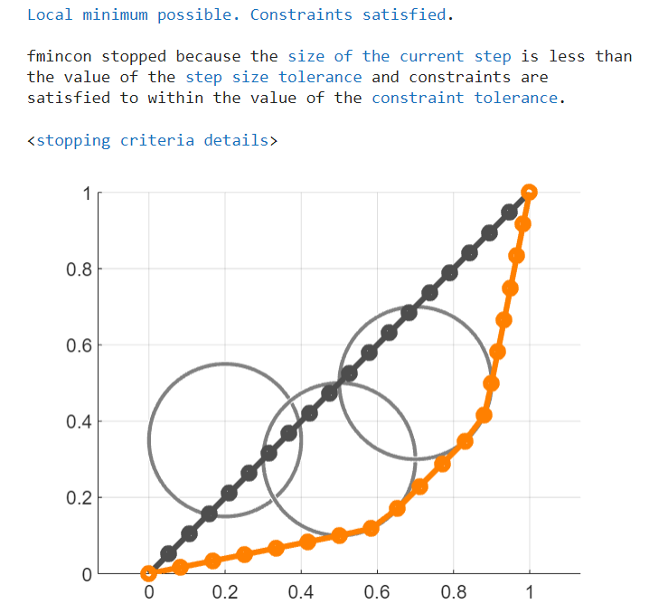
Environment 1: One obstacle with \(\normalsize center \; 𝑐_1 = [0.2, 0.35]^𝑇 \; and \; radius \; 𝑟_1 = 0.2\). A second obstacle with \(\normalsize center \; 𝑐_2 = [0.5, 0.3]^𝑇 \; and \; radius \; 𝑟_2 = 0.2\). A third obstacle with \(\normalsize center \; 𝑐_3 = [0.7, 0.5]^𝑇 \; and \; radius \; 𝑟_3 = 0.2\). Setting \(\normalsize 𝑘 = 20\).
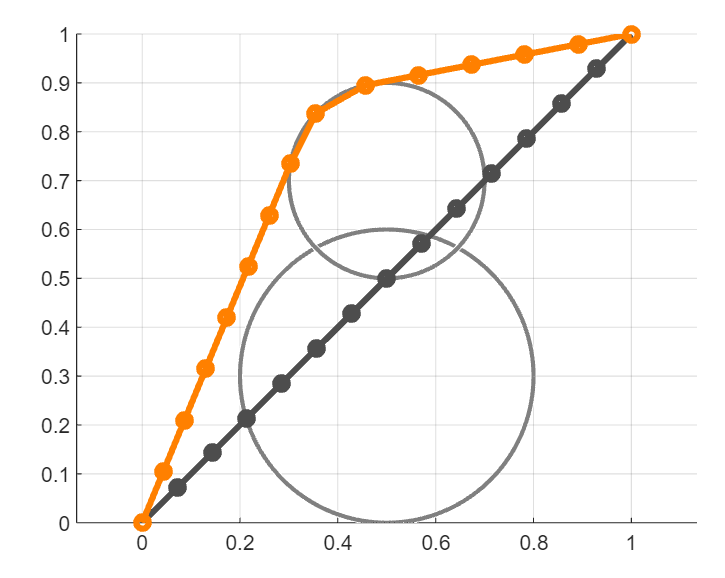
Environment 2: One obstacle with \(\normalsize center \; 𝑐_1 = [0.5, 0.3]^𝑇 \; and \; radius \; 𝑟_1 = 0.3\). A second obstacle with \(\normalsize center \; 𝑐_2 = [0.5, 0.7]^𝑇 \; and \; radius \; 𝑟_2 = 0.2\). Setting \(\normalsize 𝑘 = 15\) waypoints.
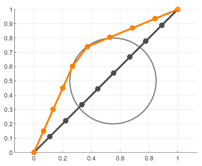
Environment 3: One obstacle with \(\normalsize center \; 𝑐_1 = [0.55, 0.5]^𝑇 \; and \; radius \; 𝑟_1 = 0.3\). Trajectory should have \(\normalsize 𝑘 = 10\) waypoints.
MATLAB Code
clearcloseall% start and goaltheta_start= [0;0];theta_goal= [1;1];centers= [0.55;0.5];radii=0.3;% initial trajectoryn=2;k=10;xi_0= [linspace(theta_start(1),theta_goal(1),k);...linspace(theta_start(2),theta_goal(2),k)];xi_0_vec=reshape(xi_0, [],1);% start and goal equality constraintsA= [eye(n) zeros(n,n*(k-1));...zeros(n,n*(k-1)),eye(n)];B= [theta_start;theta_goal];% nonlinear optimizationoptions=optimoptions('fmincon','Display','final',...'Algorithm','sqp','MaxFunctionEvaluations',1e5);xi_star_vec=fmincon(@(xi) cost(xi,centers,radii),xi_0_vec,... [], [],A,B, [], [], [],options);xi_star=reshape(xi_star_vec,2, []);% plot resultfiguregridonholdonaxisequalforidx=1:length(radii)viscircles(centers(:,idx)',radii(idx),'Color', [0.5,0.5,...0.5]);endplot(xi_0(1,:),xi_0(2,:),'o-','Color', [0.3,0.3,...0.3],'LineWidth',3);plot(xi_star(1,:),xi_star(2,:),'o-','Color', [1,0.5,...0],'LineWidth',3);% cost function to minimizefunctionC=cost(xi,centers,radii)xi=reshape(xi,2, []);C=0;foridx=2:length(xi)theta_curr=xi(:,idx);theta_prev=xi(:,idx-1);C=C+norm(theta_curr-theta_prev)^2;forjdx=1:length(radii)center=centers(:,jdx);radius=radii(jdx);ifnorm(theta_curr-center) <radiusC=C+0.5*(1/norm(theta_curr-center) -1/radius)^2;endendendend
Result:
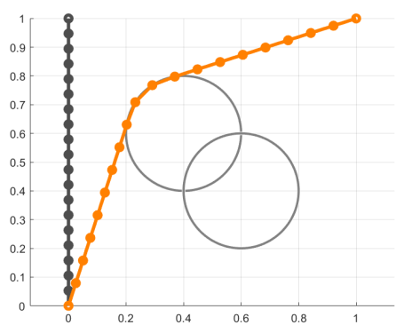
Legend: Here, in all the three environments the gray line is the initial trajectory \(\normalsize \xi^0\), while the orange line is the optimal trajectory \(\normalsize \xi\).
First obstacle with \(\normalsize center \; 𝑐_1 = [0.4, 0.6]^𝑇 \; and \; radius \; 𝑟_1 = 0.2\).
Second obstacle with \(\normalsize center \; 𝑐_2 = [0.6, 0.4]^𝑇 \; and \; radius \; 𝑟_2 = 0.2\).
The trajectory \(\normalsize \xi\) should have \(\normalsize k = 20\) waypoints.
Modifying the initial trajectory \(\normalsize \xi^0\) so that the optimal trajectory goes around both obstacles.
Solution:
For this environment an initial trajectory \(\normalsize \xi^0\) that moves straight from start to goal gets stuck. The nonlinear optimizer cannot find a way to modify this initial trajectory to decrease the cost (i.e., we are stuck in a local minima), and so the final answer simply jumps across the obstacles. We can fix this problem by choosing an initial trajectory that moves either above or below the obstacles.
This results in an optimal trajectory \(\normalsize \xi\) that goes above both obstacles. See the figure below. If we select an initial trajectory that causes the robot to converge to a path below both obstacles, that is also fine.