Inverse Kinematics Simulation

Robotics

IKO in robotics is the computational process of determining optimal joint configurations to achieve a desired end-effector pose. It plays a vital role in tasks like motion planning and control, enhancing the accuracy of robotic movements

Inverse Kinematics Optimazation

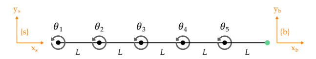
We are building a snake robot. This snake robot moves in a plane and has 5 joints, making it a redundant robot. We are using this redundancy to mimic the motion of real snakes.

Leaving \(\normalsize 𝑏 = 0\) within the Jacobian pseudoinverse. Implementing the numerical inverse kinematics algorithm to find the inverse kinematics solutions when:

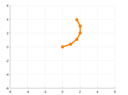
Plot of the snake robot in its initial position 𝜃 = [𝜋/8, 𝜋/8, 𝜋/8, 𝜋/8, 𝜋/8]’

Case 1: 𝐿 = 1 and the desired end-effector pose is:

\(\normalsize T_{sb} = [rotz(\pi/4), [3; 2; 0]; 0 \, 0 \, 0 \, 1]\)

Implementations

Python

Code

import numpy as np
import matplotlib
import matplotlib.pyplot as plt
matplotlib.use('Agg')  # Set the backend to a non-interactive backend
import matplotlib.animation as animation
from matplotlib.animation import PillowWriter

# Define the necessary functions
def bracket3(S):
    return np.array([[0, -S[2], S[1]], [S[2], 0, -S[0]], [-S[1], S[0], 0]])

def expm(A):
    return np.linalg.matrix_power(np.eye(A.shape[0]) + A / 16, 16)

def adjointM(T):
    R = T[0:3, 0:3]
    p = T[0:3, 3]
    return np.block([[R, np.zeros((3, 3))], [bracket3(p) @ R, R]])

def r2axisangle(R):
    if np.linalg.norm(R - np.eye(3)) < 1e-3:
        return np.array([0, 0, 0])
    else:
        theta = np.arccos(0.5 * (np.trace(R) - 1))
        omega_hat = 1 / (2 * np.sin(theta)) * (R - R.T)
        omega = np.array([omega_hat[2, 1], omega_hat[0, 2], omega_hat[1, 0]])
        return omega * theta

def bracket_s(s):
    return np.array([[0, -s[2], s[1], s[3]], [s[2], 0, -s[0], s[4]], [-s[1], s[0], 0, s[5]], [0, 0, 0, 0]])

def fk(M, S, theta):
    T = np.eye(4)
    theta = np.atleast_1d(theta)
    for i in range(len(theta)):
        T = np.dot(T, expm(bracket_s(S[:, i]) * theta[i]))
    return np.dot(T, M)

def JacS(S, theta):
    T = np.eye(4)
    Js = np.zeros((6, len(theta)))
    for i in range(len(theta)):
        Si = S[:, i]
        Js[:, i] = adjointM(T) @ Si
        T = np.dot(T, expm(bracket_s(Si) * theta[i]))
    return Js

def rotz(angle):
    c, s = np.cos(angle), np.sin(angle)
    return np.array([[c, -s, 0], [s, c, 0], [0, 0, 1]])

# Initialize plot
fig, ax = plt.subplots()
ax.set_xlim(-6, 6)
ax.set_ylim(-6, 6)
ax.grid(True)
line, = ax.plot([], [], 'o-', color=[1, 0.5, 0], linewidth=4)
plt.ion()

# Initialize parameters
L = 1
theta = np.array([np.pi/8] * 5)

S1 = np.array([0, 0, 1, 0, 0, 0])
S2 = np.array([0, 0, 1, 0, -1 * L, 0])
S3 = np.array([0, 0, 1, 0, -2 * L, 0])
S4 = np.array([0, 0, 1, 0, -3 * L, 0])
S5 = np.array([0, 0, 1, 0, -4 * L, 0])

# Create S_eq by concatenating the individual S vectors horizontally
S = np.column_stack((S1, S2, S3, S4, S5))

M = np.vstack([np.hstack([np.eye(3), np.array([[5*L, 0, 0]]).T]), [0, 0, 0, 1]])
M1 = np.vstack([np.hstack([np.eye(3), np.array([[1*L, 0, 0]]).T]), [0, 0, 0, 1]])
M2 = np.vstack([np.hstack([np.eye(3), np.array([[2*L, 0, 0]]).T]), [0, 0, 0, 1]])
M3 = np.vstack([np.hstack([np.eye(3), np.array([[3*L, 0, 0]]).T]), [0, 0, 0, 1]])
M4 = np.vstack([np.hstack([np.eye(3), np.array([[4*L, 0, 0]]).T]), [0, 0, 0, 1]])

# Desired transformation
T_d = np.vstack([np.hstack([rotz(np.pi/4), np.array([[3, 2, 0]]).T]), [0, 0, 0, 1]])
Xd = np.concatenate([r2axisangle(T_d[0:3, 0:3]), T_d[0:3, 3]])

# Initial forward kinematics
T = fk(M, S, theta)
X = np.concatenate([r2axisangle(T[0:3, 0:3]), T[0:3, 3]])

# Animation function
def update(frame):
    global theta, T, X
    if np.linalg.norm(Xd - X) > 1e-1:
        # Calculate joint transformations
        T1 = fk(M1, S[:, 0:1], theta[0])
        T2 = fk(M2, S[:, 0:2], [theta[0], theta[1]])
        T3 = fk(M3, S[:, 0:3], [theta[0], theta[1], theta[2]])
        T4 = fk(M4, S[:, 0:4], [theta[0], theta[1], theta[2], theta[3]])
        P_v = np.array([[0, 0]] + [T1[0:2, 3]]+ [T2[0:2, 3]]+ [T3[0:2, 3]]+ [T4[0:2, 3]] + [T[0:2, 3]]).T
        
        # Draw the robot
        line.set_data(P_v[0, :], P_v[1, :])
        
        # Update Jacobians and compute delta_theta
        JS = JacS(S, theta)
        Jb = np.dot(adjointM(np.linalg.inv(T)), JS)
        J_geometric = np.block([[T[0:3, 0:3], np.zeros((3, 3))], [np.zeros((3, 3)), T[0:3, 0:3]]]) @ Jb
        V = Xd - X
        delta_theta = np.dot(np.linalg.pinv(J_geometric), V)
        
        # Update theta
        theta += 0.1 * delta_theta
        print(theta)
        T = fk(M, S, theta)
        X = np.concatenate([r2axisangle(T[0:3, 0:3]), T[0:3, 3]])

    return line,

# Create and save the animation
ani = animation.FuncAnimation(fig, update, frames=np.arange(100), interval=200, blit=False)

# Save the animation
writer = PillowWriter(fps=7)  
ani.save("Inverse_Kinematics_1.gif", writer=writer)

[0.1993027  0.46598915 0.5549693  0.45091411 0.16786868]
[0.06113478 0.51001426 0.66899306 0.48188162 0.00600057]
[-0.04783409  0.54015932  0.75714363  0.5007544  -0.12217812]
[-0.13708095  0.56186278  0.82784958  0.51267239 -0.22751968]
[-0.21165874  0.57790022  0.88568751  0.52017065 -0.31583542]
[-0.27477388  0.5899323   0.93358891  0.52472423 -0.39080532]
[-0.32867117  0.59904312  0.97361294  0.5272736  -0.45499474]
[-0.37501922  0.60597918  1.00728854  0.52845196 -0.51030329]
[-0.41510644  0.61127299  1.03579107  0.52869999 -0.55819525]
[-0.4499529   0.61531389  1.06004448  0.52833026 -0.59983118]
[-0.48038014  0.61839181  1.08078598  0.52756653 -0.6361495 ]
[-0.50705787  0.62072567  1.09860977  0.52656924 -0.66792036]
[-0.53053703  0.62248263  1.11399827  0.52545283 -0.69578303]
[-0.55127405  0.62379138  1.12734533  0.52429798 -0.7202729 ]
[-0.5696494   0.62475176  1.13897385  0.52316041 -0.74184164]
[-0.5859818   0.62544159  1.14914958  0.52207742 -0.76087249]
[-0.60053959  0.62592179  1.15809195  0.52107267 -0.77769233]
[-0.61354965  0.62624023  1.16598274  0.52015989 -0.79258114]
[-0.62520472  0.62643455  1.17297302  0.51934559 -0.80577965]
[-0.63566914  0.62653443  1.17918872  0.51863112 -0.81749553]
[-0.64508373  0.62656321  1.18473524  0.51801426 -0.82790846]
[-0.65356956  0.62653929  1.18970101  0.51749037 -0.83717436]
[-0.66123122  0.62647712  1.19416061  0.5170533  -0.84542885]
[-0.66815939  0.62638801  1.19817709  0.51669598 -0.85279014]
[-0.674433    0.62628077  1.20180402  0.51641096 -0.85936152]
[-0.68012103  0.62616224  1.2050871   0.5161907  -0.86523342]
[-0.68528399  0.62603768  1.20806547  0.51602782 -0.87048512]
[-0.68997511  0.62591108  1.21077282  0.51591529 -0.87518629]
[-0.69424143  0.62578545  1.21323825  0.51584648 -0.87939821]
[-0.6981246   0.625663    1.21548703  0.51581529 -0.88317488]
[-0.70166164  0.62554531  1.21754119  0.51581611 -0.88656397]
[-0.70488554  0.62543349  1.21942004  0.51584388 -0.88960757]
[-0.70782576  0.62532823  1.22114053  0.51589405 -0.89234295]

At each iteration we first plot the robot and save a video frame. Then we calculate the Jacobian and perform numerical inverse kinematics. The loop terminates when the actual pose is close to the desired pose.

MATLAB

Code


close all
clear
clc

% create figure
figure
axis([-6, 6, -6, 6])
grid on
hold on

% save as a video file
v = VideoWriter('Inverse_Kinematics_1.mp4', 'MPEG-4');
v.FrameRate = 25;
open(v);

% initial joint values
L = 1;
theta = [pi/8; pi/8; pi/8; pi/8; pi/8];

S1 = [0 0 1 0 0 0]';
S2 = [0 0 1 0 -1*L 0]';
S3 = [0 0 1 0 -2*L 0]';
S4 = [0 0 1 0 -3*L 0]';
S5 = [0 0 1 0 -4*L 0]';

S_eq = [S1, S2, S3, S4, S5];   
M = [eye(3), [5*L;0;0]; 0 0 0 1];
M1 = [eye(3), [1*L;0;0]; 0 0 0 1];
M2 = [eye(3), [2*L;0;0]; 0 0 0 1];
M3 = [eye(3), [3*L;0;0]; 0 0 0 1];
M4 = [eye(3), [4*L;0;0]; 0 0 0 1];

% Given desired Transformation matrices T_d
T_d = [rotz(pi/4), [3;2;0]; 0 0 0 1];
Xd = [r2axisangle(T_d(1:3, 1:3)); T_d(1:3,4)];

% T with initial joint positions
T = fk(M, S_eq, theta);
X = [r2axisangle(T(1:3, 1:3)); T(1:3,4)];

while norm(Xd - X) > 1e-2

    p0 = [0; 0]; % plot the robot
    T1 = fk(M1, S1, theta(1)); % 1. get the position of each link
    T2 = fk(M2, [S1, S2], [theta(1), theta(2)]);
    T3 = fk(M3, [S1, S2, S3], [theta(1), theta(2), theta(3)]);
    T4 = fk(M4, [S1, S2, S3, S4], [theta(1), theta(2), theta(3), theta(4)]);
    P_v = [p0, T1(1:2, 4), T2(1:2, 4), T3(1:2, 4), T4(1:2, 4), T(1:2, 4)];

    cla; % 2. draw the robot and save the frame
    plot(P_v(1,:), P_v(2,:), 'o-', 'color',[1, 0.5, 0],'linewidth',4)
    drawnow
    frame = getframe(gcf);
    writeVideo(v, frame); % My Implementation for inverse kinematics calculation below

    JS = JacS(S_eq, theta); % Updated Space Jacobian
    Jb = adjointM(inv(T))*JS; %Updated Body Jacobian
    J = [T(1:3, 1:3) zeros(3); zeros(3) T(1:3, 1:3)] * Jb; % Updated Geometric Jacobian
    V = Xd - X;

    delta_theta = pinv(J)*V +(eye(5) - pinv(J)*J)*[0;0;0;0;0];

    theta = double(theta + 0.1 * delta_theta); % Updating theta until the while loop is satisfied to get the desired joint positions
    T = fk(M, S_eq, theta);
    X = [r2axisangle(T(1:3, 1:3)); T(1:3,4)];
end

close(v);
close all

Result:

Animated GIF

Case 2: 𝐿 = 1 and the desired end-effector pose is:

\(\normalsize T_{sb} = [rotz(\pi/2), [-2; 4; 0]; 0 \, 0 \, 0 \, 1]\)

Implementations

Python

Code

import numpy as np
import matplotlib
matplotlib.use('Agg')  # Set the backend to a non-interactive backend
import matplotlib.pyplot as plt
import matplotlib.animation as animation
from matplotlib.animation import PillowWriter

# Define the necessary functions
def bracket3(S):
    return np.array([[0, -S[2], S[1]], [S[2], 0, -S[0]], [-S[1], S[0], 0]])

def expm(A):
    return np.linalg.matrix_power(np.eye(A.shape[0]) + A / 16, 16)

def adjointM(T):
    R = T[0:3, 0:3]
    p = T[0:3, 3]
    return np.block([[R, np.zeros((3, 3))], [bracket3(p) @ R, R]])

def r2axisangle(R):
    if np.linalg.norm(R - np.eye(3)) < 1e-3:
        return np.array([0, 0, 0])
    else:
        theta = np.arccos(0.5 * (np.trace(R) - 1))
        omega_hat = 1 / (2 * np.sin(theta)) * (R - R.T)
        omega = np.array([omega_hat[2, 1], omega_hat[0, 2], omega_hat[1, 0]])
        return omega * theta

def bracket_s(s):
    return np.array([[0, -s[2], s[1], s[3]], [s[2], 0, -s[0], s[4]], [-s[1], s[0], 0, s[5]], [0, 0, 0, 0]])

def fk(M, S, theta):
    T = np.eye(4)
    theta = np.atleast_1d(theta)
    for i in range(len(theta)):
        T = np.dot(T, expm(bracket_s(S[:, i]) * theta[i]))
    return np.dot(T, M)

def JacS(S, theta):
    T = np.eye(4)
    Js = np.zeros((6, len(theta)))
    for i in range(len(theta)):
        Si = S[:, i]
        Js[:, i] = np.dot(adjointM(T), Si)
        T = np.dot(T, expm(bracket_s(Si) * theta[i]))
    return Js

def rotz(angle):
    c, s = np.cos(angle), np.sin(angle)
    return np.array([[c, -s, 0], [s, c, 0], [0, 0, 1]])

# Initialize plot
fig, ax = plt.subplots()
ax.set_xlim(-6, 6)
ax.set_ylim(-6, 6)
ax.grid(True)
line, = ax.plot([], [], 'o-', color=[1, 0.5, 0], linewidth=4)
plt.ion()

# Initialize parameters
L = 1
theta = np.array([np.pi/8] * 5)

S1 = np.array([0, 0, 1, 0, 0, 0])
S2 = np.array([0, 0, 1, 0, -1 * L, 0])
S3 = np.array([0, 0, 1, 0, -2 * L, 0])
S4 = np.array([0, 0, 1, 0, -3 * L, 0])
S5 = np.array([0, 0, 1, 0, -4 * L, 0])

# Create S_eq by concatenating the individual S vectors horizontally
S = np.column_stack((S1, S2, S3, S4, S5))

M = np.vstack([np.hstack([np.eye(3), np.array([[5*L, 0, 0]]).T]), [0, 0, 0, 1]])
M1 = np.vstack([np.hstack([np.eye(3), np.array([[1*L, 0, 0]]).T]), [0, 0, 0, 1]])
M2 = np.vstack([np.hstack([np.eye(3), np.array([[2*L, 0, 0]]).T]), [0, 0, 0, 1]])
M3 = np.vstack([np.hstack([np.eye(3), np.array([[3*L, 0, 0]]).T]), [0, 0, 0, 1]])
M4 = np.vstack([np.hstack([np.eye(3), np.array([[4*L, 0, 0]]).T]), [0, 0, 0, 1]])

# Desired transformation
T_d = np.vstack([np.hstack([rotz(np.pi/2), np.array([[-2, 4, 0]]).T]), [0, 0, 0, 1]])
Xd = np.concatenate([r2axisangle(T_d[0:3, 0:3]), T_d[0:3, 3]])

# Initial forward kinematics
T = fk(M, S, theta)
X = np.concatenate([r2axisangle(T[0:3, 0:3]), T[0:3, 3]])

# Animation function
def update(frame):
    global theta, T, X
    if np.linalg.norm(Xd - X) > 1e-1:
        # Calculate joint transformations
        T1 = fk(M1, S[:, 0:1], theta[0])
        T2 = fk(M2, S[:, 0:2], [theta[0], theta[1]])
        T3 = fk(M3, S[:, 0:3], [theta[0], theta[1], theta[2]])
        T4 = fk(M4, S[:, 0:4], [theta[0], theta[1], theta[2], theta[3]])
        P_v = np.array([[0, 0]] + [T1[0:2, 3]]+ [T2[0:2, 3]]+ [T3[0:2, 3]]+ [T4[0:2, 3]] + [T[0:2, 3]]).T
        
        # Draw the robot
        line.set_data(P_v[0, :], P_v[1, :])
        
        # Update Jacobians and compute delta_theta
        JS = JacS(S, theta)
        Jb = np.dot(adjointM(np.linalg.inv(T)), JS)
        J_geometric = np.block([[T[0:3, 0:3], np.zeros((3, 3))], [np.zeros((3, 3)), T[0:3, 0:3]]]) @ Jb
        V = Xd - X
        delta_theta = np.dot(np.linalg.pinv(J_geometric), V)
        
        # Update theta
        theta += 0.1 * delta_theta
        print(theta)
        T = fk(M, S, theta)
        X = np.concatenate([r2axisangle(T[0:3, 0:3]), T[0:3, 3]])

    return line,

# Create and save the animation
ani = animation.FuncAnimation(fig, update, frames=np.arange(100), interval=200, blit=False)

# Save the animation
writer = PillowWriter(fps=7)  
ani.save("Inverse_Kinematics_2.gif", writer=writer)

[0.27558403 0.52539357 0.58147356 0.43337151 0.10176109]
[ 0.23291267  0.62281115  0.69826779  0.42871219 -0.10691892]
[ 0.22580829  0.70313343  0.77671288  0.40497409 -0.27382697]
[ 0.24119701  0.77132002  0.82821562  0.37105773 -0.41150535]
[ 0.2718153   0.8295479   0.85923151  0.33181449 -0.52627559]
[ 0.31274707  0.87904332  0.8743584   0.2903601  -0.62219375]
[ 0.36037301  0.92067736  0.8772505   0.24879702 -0.70229657]
[ 0.41195291  0.95520389  0.8709295   0.2085294  -0.76907122]
[ 0.46541083  0.98335279  0.85790084  0.17044848 -0.82464119]
[ 0.51919361  1.00585499  0.84021288  0.13506709 -0.870841  ]
[ 0.5721616   1.02343655  0.81950593  0.10262535 -0.90925052]
[ 0.62349983  1.03680166  0.79706383  0.07317388 -0.94121782]
[ 0.67264561  1.04661494  0.77386781  0.04663753 -0.96788097]
[ 0.71923024  1.05348758  0.75064905  0.02286273 -0.99019128]
[ 0.7630329   1.05796872  0.72793692  0.00165141 -1.00893724]
[ 0.8039445   1.06054162  0.70610121 -0.01721531 -1.02476784]
[ 0.84193941  1.06162373  0.68538768 -0.03396117 -1.03821437]
[ 0.87705364  1.0615696   0.66594718 -0.04880443 -1.04970985]
[ 0.90936772  1.06067554  0.64785912 -0.06195155 -1.05960604]
[ 0.93899362  1.05918532  0.63114996 -0.07359367 -1.06818794]
[ 0.96606452  1.05729631  0.61580777 -0.08390494 -1.07568598]
[ 0.9907269   1.05516563  0.60179336 -0.09304224 -1.08228624]
[ 1.01313455  1.05291598  0.58904898 -0.10114556 -1.08813882]
[ 1.0334439   1.05064118  0.57750482 -0.10833905 -1.09336475]
[ 1.05181053  1.04841102  0.567084   -0.11473216 -1.09806168]
[ 1.06838657  1.04627563  0.55770621 -0.12042109 -1.10230846]
[ 1.08331882  1.04426933  0.5492905  -0.1254901  -1.10616887]
[ 1.09674737  1.04241382  0.54175722 -0.13001288 -1.10969466]
[ 1.10880476  1.04072101  0.53502938 -0.13405379 -1.11292799]
[ 1.1196154   1.03919526  0.52903362 -0.13766903 -1.11590337]
[ 1.12929533  1.03783535  0.52370084 -0.14090766 -1.11864926]
[ 1.13795221  1.03663596  0.51896646 -0.14381257 -1.12118929]
[ 1.14568536  1.03558894  0.51477065 -0.14642125 -1.12354325]
[ 1.15258609  1.0346843   0.51105826 -0.14876653 -1.12572791]
[ 1.15873796  1.03391096  0.50777879 -0.15087723 -1.12775764]

MATLAB

Code


close all
clear
clc

% create figure
figure
axis([-6, 6, -6, 6])
grid on
hold on

% save as a video file
v = VideoWriter('Inverse_Kinematics_2.mp4', 'MPEG-4');
v.FrameRate = 25;
open(v);

% initial joint values
L = 1;
theta = [pi/8; pi/8; pi/8; pi/8; pi/8];

S1 = [0 0 1 0 0 0]';
S2 = [0 0 1 0 -1*L 0]';
S3 = [0 0 1 0 -2*L 0]';
S4 = [0 0 1 0 -3*L 0]';
S5 = [0 0 1 0 -4*L 0]';

S_eq = [S1, S2, S3, S4, S5];   
M = [eye(3), [5*L;0;0]; 0 0 0 1];
M1 = [eye(3), [1*L;0;0]; 0 0 0 1];
M2 = [eye(3), [2*L;0;0]; 0 0 0 1];
M3 = [eye(3), [3*L;0;0]; 0 0 0 1];
M4 = [eye(3), [4*L;0;0]; 0 0 0 1];

% Given desired Transformation matrices T_d
T_d = [rotz(pi/4), [-2;4;0]; 0 0 0 1];
Xd = [r2axisangle(T_d(1:3, 1:3)); T_d(1:3,4)];

% T with initial joint positions
T = fk(M, S_eq, theta);
X = [r2axisangle(T(1:3, 1:3)); T(1:3,4)];

while norm(Xd - X) > 1e-2

    p0 = [0; 0]; % plot the robot
    T1 = fk(M1, S1, theta(1)); % 1. get the position of each link
    T2 = fk(M2, [S1, S2], [theta(1), theta(2)]);
    T3 = fk(M3, [S1, S2, S3], [theta(1), theta(2), theta(3)]);
    T4 = fk(M4, [S1, S2, S3, S4], [theta(1), theta(2), theta(3), theta(4)]);
    P_v = [p0, T1(1:2, 4), T2(1:2, 4), T3(1:2, 4), T4(1:2, 4), T(1:2, 4)];

    cla; % 2. draw the robot and save the frame
    plot(P_v(1,:), P_v(2,:), 'o-', 'color',[1, 0.5, 0],'linewidth',4)
    drawnow
    frame = getframe(gcf);
    writeVideo(v, frame); % My Implementation for inverse kinematics calculation below

    JS = JacS(S_eq, theta); % Updated Space Jacobian
    Jb = adjointM(inv(T))*JS; %Updated Body Jacobian
    J = [T(1:3, 1:3) zeros(3); zeros(3) T(1:3, 1:3)] * Jb; % Updated Geometric Jacobian
    V = Xd - X;

    delta_theta = pinv(J)*V +(eye(5) - pinv(J)*J)*[0;0;0;0;0];

    theta = double(theta + 0.1 * delta_theta); % Updating theta until the while loop is satisfied to get the desired joint positions
    T = fk(M, S_eq, theta);
    X = [r2axisangle(T(1:3, 1:3)); T(1:3,4)];
end

close(v);
close all

Result:

Animated GIF

Case 3: 𝐿 = 1 and the desired end-effector pose is:

\(\normalsize T_{sb} = [rotz(0), [3; -1; 0]; 0 \, 0 \, 0 \, 1]\)

Implementations

Python

Code

import numpy as np
import matplotlib
matplotlib.use('Agg')  # Set the backend to a non-interactive backend
import matplotlib.pyplot as plt
import matplotlib.animation as animation
from matplotlib.animation import PillowWriter

# Define the necessary functions
def bracket3(S):
    return np.array([[0, -S[2], S[1]], [S[2], 0, -S[0]], [-S[1], S[0], 0]])

def expm(A):
    return np.linalg.matrix_power(np.eye(A.shape[0]) + A / 16, 16)

def adjointM(T):
    R = T[0:3, 0:3]
    p = T[0:3, 3]
    return np.block([[R, np.zeros((3, 3))], [bracket3(p) @ R, R]])

def r2axisangle(R):
    if np.linalg.norm(R - np.eye(3)) < 1e-3:
        return np.array([0, 0, 0])
    else:
        trace = np.clip((np.trace(R) - 1) / 2, -1, 1)  # Clip trace to the valid range
        if trace < -1:
            trace = -1
        elif trace > 1:
            trace = 1
        theta = np.arccos(0.5*trace)
        omega_hat = 1 / (2 * np.sin(theta)) * (R - R.T)
        omega = np.array([omega_hat[2, 1], omega_hat[0, 2], omega_hat[1, 0]])
        return omega * theta

def bracket_s(s):
    return np.array([[0, -s[2], s[1], s[3]], [s[2], 0, -s[0], s[4]], [-s[1], s[0], 0, s[5]], [0, 0, 0, 0]])

def fk(M, S, theta):
    T = np.eye(4)
    theta = np.atleast_1d(theta)
    for i in range(len(theta)):
        T = np.dot(T, expm(bracket_s(S[:, i]) * theta[i]))
    return np.dot(T, M)

def JacS(S, theta):
    T = np.eye(4)
    Js = np.zeros((6, len(theta)))
    for i in range(len(theta)):
        Si = S[:, i]
        Js[:, i] = np.dot(adjointM(T), Si)
        T = np.dot(T, expm(bracket_s(Si) * theta[i]))
    return Js

def rotz(angle):
    c, s = np.cos(angle), np.sin(angle)
    return np.array([[c, -s, 0], [s, c, 0], [0, 0, 1]])

# Initialize plot
fig, ax = plt.subplots()
ax.set_xlim(-6, 6)
ax.set_ylim(-6, 6)
ax.grid(True)
line, = ax.plot([], [], 'o-', color=[1, 0.5, 0], linewidth=4)
plt.ion()

# Initialize parameters
L = 1
theta = np.array([np.pi/8] * 5)

S1 = np.array([0, 0, 1, 0, 0, 0])
S2 = np.array([0, 0, 1, 0, -1 * L, 0])
S3 = np.array([0, 0, 1, 0, -2 * L, 0])
S4 = np.array([0, 0, 1, 0, -3 * L, 0])
S5 = np.array([0, 0, 1, 0, -4 * L, 0])

# Create S_eq by concatenating the individual S vectors horizontally
S = np.column_stack((S1, S2, S3, S4, S5))

M = np.vstack([np.hstack([np.eye(3), np.array([[5*L, 0, 0]]).T]), [0, 0, 0, 1]])
M1 = np.vstack([np.hstack([np.eye(3), np.array([[1*L, 0, 0]]).T]), [0, 0, 0, 1]])
M2 = np.vstack([np.hstack([np.eye(3), np.array([[2*L, 0, 0]]).T]), [0, 0, 0, 1]])
M3 = np.vstack([np.hstack([np.eye(3), np.array([[3*L, 0, 0]]).T]), [0, 0, 0, 1]])
M4 = np.vstack([np.hstack([np.eye(3), np.array([[4*L, 0, 0]]).T]), [0, 0, 0, 1]])

# Desired transformation
T_d = np.vstack([np.hstack([rotz(0), np.array([[3, -1, 0]]).T]), [0, 0, 0, 1]])
Xd = np.concatenate([r2axisangle(T_d[0:3, 0:3]), T_d[0:3, 3]])

# Initial forward kinematics
T = fk(M, S, theta)
X = np.concatenate([r2axisangle(T[0:3, 0:3]), T[0:3, 3]])

# Animation function
def update(frame):
    global theta, T, X
    if np.linalg.norm(Xd - X) > 1e-1:
        # Calculate joint transformations
        T1 = fk(M1, S[:, 0:1], theta[0])
        T2 = fk(M2, S[:, 0:2], [theta[0], theta[1]])
        T3 = fk(M3, S[:, 0:3], [theta[0], theta[1], theta[2]])
        T4 = fk(M4, S[:, 0:4], [theta[0], theta[1], theta[2], theta[3]])
        P_v = np.array([[0, 0]] + [T1[0:2, 3]]+ [T2[0:2, 3]]+ [T3[0:2, 3]]+ [T4[0:2, 3]] + [T[0:2, 3]]).T
        
        # Draw the robot
        line.set_data(P_v[0, :], P_v[1, :])
        
        # Update Jacobians and compute delta_theta
        JS = JacS(S, theta)
        Jb = np.dot(adjointM(np.linalg.inv(T)), JS)
        J_geometric = np.block([[T[0:3, 0:3], np.zeros((3, 3))], [np.zeros((3, 3)), T[0:3, 0:3]]]) @ Jb
        V = Xd - X
        delta_theta = np.dot(np.linalg.pinv(J_geometric), V)
        
        # Update theta
        theta += 0.1 * delta_theta
        print(theta)
        T = fk(M, S, theta)
        X = np.concatenate([r2axisangle(T[0:3, 0:3]), T[0:3, 3]])

    return line,

# Create and save the animation
ani = animation.FuncAnimation(fig, update, frames=np.arange(100), interval=200, blit=False)

# Save the animation
writer = PillowWriter(fps=7)  
ani.save("Inverse_Kinematics_3.gif", writer=writer)

[-0.05314555  0.56290261  0.78072182  0.56314343 -0.06077186]
[-0.33026032  0.63092663  1.01551888  0.63990985 -0.33531103]
[-0.55313051  0.66623181  1.19775149  0.69005746 -0.55022883]
[-0.74036733  0.68131901  1.34397836  0.72586206 -0.72416418]
[-0.899747    0.68214433  1.46120003  0.75317194 -0.86472893]
[-1.03582782  0.67258771  1.55378335  0.77545496 -0.97669791]
[-1.1519017   0.65561888  1.62525653  0.79481972 -1.06406388]
[-1.25062936  0.63367531  1.6788238   0.81244052 -1.13056494]
[-1.33428373  0.60877274  1.71746794  0.82885285 -1.1797263 ]
[-1.40486005  0.58256283  1.74395497  0.84415241 -1.21486659]
[-1.46406795  0.55687648  1.76118173  0.85743896 -1.24027725]
[-1.51353785  0.53217219  1.77100399  0.86915723 -1.25745585]
[-1.55474869  0.50873305  1.77503385  0.87962813 -1.26781729]
[-1.58900369  0.4867206   1.77463151  0.8890719  -1.27265526]
[-1.61742724  0.46621157  1.77091752  0.8976355  -1.27311668]
[-1.6409756   0.44722316  1.76479726  0.90541746 -1.2701912 ]
[-1.66045459  0.42973107  1.75699074  0.91248714 -1.26471358]
[-1.67653945  0.4136828   1.74806283  0.9188978  -1.25737455]
[-1.68979423  0.39900764  1.73845126  0.92469464 -1.24873636]
[-1.7006894   0.38562402  1.72849118  0.9299192  -1.23925005]
[-1.70961713  0.37344497  1.71843577  0.93461151 -1.22927246]
[-1.71690439  0.36238196  1.70847343  0.93881083 -1.21908203]
[-1.72282384  0.35234764  1.69874154  0.9425557  -1.20889267]
[-1.72760309  0.34325763  1.68933768  0.94588371 -1.19886582]
[-1.73143222  0.3350316   1.68032849  0.94883113 -1.18912055]
[-1.73447014  0.327594    1.67175674  0.95143261 -1.17974204]
[-1.73684978  0.32087437  1.6636469   0.95372086 -1.17078857]
[-1.73868244  0.31480739  1.65600958  0.95572658 -1.16229719]
[-1.74006138  0.30933284  1.64884495  0.95747827 -1.15428843]
[-1.74106475  0.3043954   1.64214551  0.95900226 -1.14677005]
[-1.74175811  0.29994445  1.6358982   0.96032272 -1.13974006]
[-1.74219649  0.29593375  1.63008604  0.96146173 -1.13318921]
[-1.74242602  0.29232115  1.62468945  0.9624394  -1.12710291]
[-1.74248544  0.28906833  1.61968724  0.96327395 -1.12146281]
[-1.74240725  0.28614046  1.61505735  0.96398183 -1.11624799]
[-1.74221868  0.28350593  1.61077745  0.96457789 -1.11143595]
[-1.74194258  0.2811361   1.60682536  0.96507547 -1.10700338]
[-1.74159806  0.279005    1.60317935  0.96548656 -1.10292668]
[-1.74120108  0.27708916  1.59981843  0.96582187 -1.09918245]

MATLAB

Code


close all
clear
clc

% create figure
figure
axis([-6, 6, -6, 6])
grid on
hold on

% save as a video file
v = VideoWriter('Inverse_Kinematics_3.mp4', 'MPEG-4');
v.FrameRate = 25;
open(v);

% initial joint values
L = 1;
theta = [pi/8; pi/8; pi/8; pi/8; pi/8];

S1 = [0 0 1 0 0 0]';
S2 = [0 0 1 0 -1*L 0]';
S3 = [0 0 1 0 -2*L 0]';
S4 = [0 0 1 0 -3*L 0]';
S5 = [0 0 1 0 -4*L 0]';

S_eq = [S1, S2, S3, S4, S5];   
M = [eye(3), [5*L;0;0]; 0 0 0 1];
M1 = [eye(3), [1*L;0;0]; 0 0 0 1];
M2 = [eye(3), [2*L;0;0]; 0 0 0 1];
M3 = [eye(3), [3*L;0;0]; 0 0 0 1];
M4 = [eye(3), [4*L;0;0]; 0 0 0 1];

% Given desired Transformation matrices T_d
T_d = [rotz(0), [3;-1;0]; 0 0 0 1];
Xd = [r2axisangle(T_d(1:3, 1:3)); T_d(1:3,4)];

% T with initial joint positions
T = fk(M, S_eq, theta);
X = [r2axisangle(T(1:3, 1:3)); T(1:3,4)];

while norm(Xd - X) > 1e-2

    p0 = [0; 0]; % plot the robot
    T1 = fk(M1, S1, theta(1)); % 1. get the position of each link
    T2 = fk(M2, [S1, S2], [theta(1), theta(2)]);
    T3 = fk(M3, [S1, S2, S3], [theta(1), theta(2), theta(3)]);
    T4 = fk(M4, [S1, S2, S3, S4], [theta(1), theta(2), theta(3), theta(4)]);
    P_v = [p0, T1(1:2, 4), T2(1:2, 4), T3(1:2, 4), T4(1:2, 4), T(1:2, 4)];

    cla; % 2. draw the robot and save the frame
    plot(P_v(1,:), P_v(2,:), 'o-', 'color',[1, 0.5, 0],'linewidth',4)
    drawnow
    frame = getframe(gcf);
    writeVideo(v, frame); % My Implementation for inverse kinematics calculation below

    JS = JacS(S_eq, theta); % Updated Space Jacobian
    Jb = adjointM(inv(T))*JS; %Updated Body Jacobian
    J = [T(1:3, 1:3) zeros(3); zeros(3) T(1:3, 1:3)] * Jb; % Updated Geometric Jacobian
    V = Xd - X;

    delta_theta = pinv(J)*V +(eye(5) - pinv(J)*J)*[0;0;0;0;0];

    theta = double(theta + 0.1 * delta_theta); % Updating theta until the while loop is satisfied to get the desired joint positions
    T = fk(M, S_eq, theta);
    X = [r2axisangle(T(1:3, 1:3)); T(1:3,4)];
end

close(v);
close all

Result:

Animated GIF

Jacobian Pseudoinverse and Redundancy

This problem continues exploring the redundant snake robot used simulated above. So far we have left \(\normalsize 𝑏 = 0\) in our Jacobian pseudoinverse. More generally, choosing \(\normalsize 𝑏\) allows us to set a secondary objective for the inverse kinematics of redundant robots.

Here we establish that numerical inverse kinematics finds a solution for \(\normalsize \theta\) such that \(\normalsize T_{sb}(\theta)\) equals the desired end-effector pose. But when working with redundant robots, multiple solutions are often possible. Choosing \(\normalsize 𝑏\) affects which of these solutions the algorithm selects.

Now I set \(\normalsize 𝑏\) as the following vector (and update \(\normalsize 𝑏\) as \(\normalsize \theta_1\) changes):

\[\normalsize b = \left(\begin{array}{cc} -\theta_1(0)\\ 0\\ 0\\ 0\\ 0\\ \end{array}\right) \]

Which is a \(\normalsize (6 * 1) \, vector\)

Equation: \(\normalsize \delta\theta = pinv(J)*V + (I - pinv(J)*J)*b\)

Here we change the delta_theta by manipulating the pseudoinverse and introducing the null-space

Note: \(\normalsize 𝑏\) was a zero vector till now for all the three cases, but now we will notice the change for Case 3:

CASE 3: Modified delta_theta for Redundancy

Implementations

Python

Code

import numpy as np
import matplotlib
matplotlib.use('Agg')  # Set the backend to a non-interactive backend
import matplotlib.pyplot as plt
import matplotlib.animation as animation
from matplotlib.animation import PillowWriter

# Define the necessary functions
def bracket3(S):
    return np.array([[0, -S[2], S[1]], [S[2], 0, -S[0]], [-S[1], S[0], 0]])

def expm(A):
    return np.linalg.matrix_power(np.eye(A.shape[0]) + A / 16, 16)

def adjointM(T):
    R = T[0:3, 0:3]
    p = T[0:3, 3]
    return np.block([[R, np.zeros((3, 3))], [bracket3(p) @ R, R]])

def r2axisangle(R):
    if np.linalg.norm(R - np.eye(3)) < 1e-3:
        return np.array([0, 0, 0])
    else:
        trace = np.clip((np.trace(R) - 1) / 2, -1, 1)  # Clip trace to the valid range
        if trace < -1:
            trace = -1
        elif trace > 1:
            trace = 1
        theta = np.arccos(0.5*trace)
        omega_hat = 1 / (2 * np.sin(theta)) * (R - R.T)
        omega = np.array([omega_hat[2, 1], omega_hat[0, 2], omega_hat[1, 0]])
        return omega * theta

def bracket_s(s):
    return np.array([[0, -s[2], s[1], s[3]], [s[2], 0, -s[0], s[4]], [-s[1], s[0], 0, s[5]], [0, 0, 0, 0]])

def fk(M, S, theta):
    T = np.eye(4)
    theta = np.atleast_1d(theta)
    for i in range(len(theta)):
        T = np.dot(T, expm(bracket_s(S[:, i]) * theta[i]))
    return np.dot(T, M)

def JacS(S, theta):
    T = np.eye(4)
    Js = np.zeros((6, len(theta)))
    for i in range(len(theta)):
        Si = S[:, i]
        Js[:, i] = np.dot(adjointM(T), Si)
        T = np.dot(T, expm(bracket_s(Si) * theta[i]))
    return Js

def rotz(angle):
    c, s = np.cos(angle), np.sin(angle)
    return np.array([[c, -s, 0], [s, c, 0], [0, 0, 1]])

# Initialize plot
fig, ax = plt.subplots()
ax.set_xlim(-6, 6)
ax.set_ylim(-6, 6)
ax.grid(True)
line, = ax.plot([], [], 'o-', color=[1, 0.5, 0], linewidth=4)
plt.ion()

# Initialize parameters
L = 1
theta = np.array([np.pi/8] * 5)

S1 = np.array([0, 0, 1, 0, 0, 0])
S2 = np.array([0, 0, 1, 0, -1 * L, 0])
S3 = np.array([0, 0, 1, 0, -2 * L, 0])
S4 = np.array([0, 0, 1, 0, -3 * L, 0])
S5 = np.array([0, 0, 1, 0, -4 * L, 0])

# Create S_eq by concatenating the individual S vectors horizontally
S = np.column_stack((S1, S2, S3, S4, S5))

M = np.vstack([np.hstack([np.eye(3), np.array([[5*L, 0, 0]]).T]), [0, 0, 0, 1]])
M1 = np.vstack([np.hstack([np.eye(3), np.array([[1*L, 0, 0]]).T]), [0, 0, 0, 1]])
M2 = np.vstack([np.hstack([np.eye(3), np.array([[2*L, 0, 0]]).T]), [0, 0, 0, 1]])
M3 = np.vstack([np.hstack([np.eye(3), np.array([[3*L, 0, 0]]).T]), [0, 0, 0, 1]])
M4 = np.vstack([np.hstack([np.eye(3), np.array([[4*L, 0, 0]]).T]), [0, 0, 0, 1]])

# Desired transformation
T_d = np.vstack([np.hstack([rotz(0), np.array([[3, -1, 0]]).T]), [0, 0, 0, 1]])
Xd = np.concatenate([r2axisangle(T_d[0:3, 0:3]), T_d[0:3, 3]])

# Initial forward kinematics
T = fk(M, S, theta)
X = np.concatenate([r2axisangle(T[0:3, 0:3]), T[0:3, 3]])

# Animation function
def update(frame):
    global theta, T, X
    if np.linalg.norm(Xd - X) > 1e-1:
        # Calculate joint transformations
        T1 = fk(M1, S[:, 0:1], theta[0])
        T2 = fk(M2, S[:, 0:2], [theta[0], theta[1]])
        T3 = fk(M3, S[:, 0:3], [theta[0], theta[1], theta[2]])
        T4 = fk(M4, S[:, 0:4], [theta[0], theta[1], theta[2], theta[3]])
        P_v = np.array([[0, 0]] + [T1[0:2, 3]]+ [T2[0:2, 3]]+ [T3[0:2, 3]]+ [T4[0:2, 3]] + [T[0:2, 3]]).T
        
        # Draw the robot
        line.set_data(P_v[0, :], P_v[1, :])
        
        # Update Jacobians and compute delta_theta
        JS = JacS(S, theta)
        Jb = np.dot(adjointM(np.linalg.inv(T)), JS)
        J_geometric = np.block([[T[0:3, 0:3], np.zeros((3, 3))], [np.zeros((3, 3)), T[0:3, 0:3]]]) @ Jb
        V = Xd - X

        # [del_theta = pinv(J)*V + (I - pinv(J)*J)*b] <- Updated delta_theta to include the null-space with the specified b vector
        delta_theta = np.dot(np.linalg.pinv(J_geometric), V) + np.dot((np.eye(5) - np.dot(np.linalg.pinv(J_geometric), J_geometric)), np.array([-theta[0], 0, 0, 0, 0]))
        
        # Update theta
        theta += 0.1 * delta_theta
        print(theta)
        T = fk(M, S, theta)
        X = np.concatenate([r2axisangle(T[0:3, 0:3]), T[0:3, 3]])

    return line,

# Create and save the animation
ani = animation.FuncAnimation(fig, update, frames=np.arange(100), interval=200, blit=False)

# Save the animation
writer = PillowWriter(fps=7)  
ani.save("Inverse_Kinematics_Null.gif", writer=writer)

[-0.05825544  0.57353743  0.77725608  0.55724953 -0.05693715]
[-0.33556013  0.64086137  1.01264325  0.63447309 -0.33163482]
[-0.55265956  0.6656847   1.19866303  0.68949924 -0.55051267]
[-0.72772164  0.6618604   1.35115636  0.73355974 -0.73223516]
[-0.86867406  0.63683335  1.47639744  0.77174108 -0.88425018]
[-0.98076153  0.59594891  1.57808655  0.80704634 -1.01096916]
[-1.06833973  0.54347282  1.65917606  0.8414017  -1.11585497]
[-1.1353063   0.48290628  1.72238131  0.87600273 -1.20200833]
[-1.18514846  0.41710933  1.77026723  0.91149258 -1.27228264]
[-1.2209048   0.34840453  1.80524701  0.9480471  -1.32935905]
[-1.24502034  0.27912295  1.8300012   0.98468336 -1.37700902]
[-1.25970342  0.21019292  1.84615904  1.02171894 -1.41627532]
[-1.26680285  0.14229845  1.85516799  1.05926318 -1.44822922]
[-1.26782221  0.07593138  1.85828783  1.09726722 -1.47392191]
[-1.2639633   0.01142763  1.85659734  1.13558306 -1.49433971]
[-1.25618019 -0.05100306  1.85100817  1.17401545 -1.510373  ]
[-1.24523121 -0.11125002  1.84228215  1.21235971 -1.52280077]
[-1.23172299 -0.16927717  1.83104994  1.25042495 -1.53228789]
[-1.2161452  -0.22510185  1.81782933  1.2880459  -1.53939092]
[-1.19889701 -0.27877757  1.80304255  1.32508688 -1.54456879]
[-1.18030676 -0.3303806   1.7870319   1.36144127 -1.54819533]
[-1.16064685 -0.38000008  1.77007342  1.39702856 -1.55057206]
[-1.14014478 -0.42773089  1.75238878  1.4317905  -1.55193998]
[-1.1189917  -0.47366884  1.73415522  1.46568709 -1.55249019]
[-1.09734903 -0.51790738  1.71551396  1.49869293 -1.55237297]
[-1.07535365 -0.56053566  1.69657713  1.530794   -1.55170554]
[-1.0531221  -0.60163728  1.6774335   1.56198494 -1.55057842]
[-1.0307539  -0.64128977  1.65815321  1.59226689 -1.54906086]
[-1.00833432 -0.67956441  1.63879161  1.62164574 -1.54720524]
[-0.98593665 -0.71652631  1.61939242  1.65013075 -1.54505065]
[-0.96362401 -0.75223473  1.59999035  1.67773349 -1.54262592]
[-0.9414509  -0.78674343  1.58061313  1.7044671  -1.53995205]
[-0.91946448 -0.8201012   1.56128328  1.73034568 -1.53704415]
[-0.89770558 -0.8523523   1.54201945  1.75538388 -1.5339131 ]
[-0.87620958 -0.88353702  1.52283751  1.7795967  -1.53056685]
[-0.8550071  -0.91369218  1.50375142  1.80299926 -1.52701146]
[-0.83412458 -0.94285159  1.48477389  1.82560676 -1.52325189]
[-0.81358477 -0.97104661  1.46591687  1.84743444 -1.5192927 ]
[-0.79340707 -0.9983065   1.44719191  1.8684976  -1.51513849]
[-0.77360792 -1.02465885  1.42861042  1.88881166 -1.51079429]
[-0.75420097 -1.05012997  1.41018377  1.90839219 -1.50626577]
[-0.73519738 -1.07474516  1.39192337  1.927255   -1.50155939]

MATLAB

Code


close all
clear
clc

% create figure
figure
axis([-6, 6, -6, 6])
grid on
hold on

% save as a video file
v = VideoWriter('Inverse_Kinematics_3_null_space.mp4', 'MPEG-4');
v.FrameRate = 25;
open(v);

% initial joint values
L = 1;
theta = [pi/8; pi/8; pi/8; pi/8; pi/8];

S1 = [0 0 1 0 0 0]';
S2 = [0 0 1 0 -1*L 0]';
S3 = [0 0 1 0 -2*L 0]';
S4 = [0 0 1 0 -3*L 0]';
S5 = [0 0 1 0 -4*L 0]';

S_eq = [S1, S2, S3, S4, S5];   
M = [eye(3), [5*L;0;0]; 0 0 0 1];
M1 = [eye(3), [1*L;0;0]; 0 0 0 1];
M2 = [eye(3), [2*L;0;0]; 0 0 0 1];
M3 = [eye(3), [3*L;0;0]; 0 0 0 1];
M4 = [eye(3), [4*L;0;0]; 0 0 0 1];

% Given desired Transformation matrices T_d
T_d = [rotz(0), [3;-1;0]; 0 0 0 1];
Xd = [r2axisangle(T_d(1:3, 1:3)); T_d(1:3,4)];

% T with initial joint positions
T = fk(M, S_eq, theta);
X = [r2axisangle(T(1:3, 1:3)); T(1:3,4)];

while norm(Xd - X) > 1e-2

    p0 = [0; 0]; % plot the robot
    T1 = fk(M1, S1, theta(1)); % 1. get the position of each link
    T2 = fk(M2, [S1, S2], [theta(1), theta(2)]);
    T3 = fk(M3, [S1, S2, S3], [theta(1), theta(2), theta(3)]);
    T4 = fk(M4, [S1, S2, S3, S4], [theta(1), theta(2), theta(3), theta(4)]);
    P_v = [p0, T1(1:2, 4), T2(1:2, 4), T3(1:2, 4), T4(1:2, 4), T(1:2, 4)];

    cla; % 2. draw the robot and save the frame
    plot(P_v(1,:), P_v(2,:), 'o-', 'color',[1, 0.5, 0],'linewidth',4)
    drawnow
    frame = getframe(gcf);
    writeVideo(v, frame); % My Implementation for inverse kinematics calculation below

    JS = JacS(S_eq, theta); % Updated Space Jacobian
    Jb = adjointM(inv(T))*JS; %Updated Body Jacobian
    J = [T(1:3, 1:3) zeros(3); zeros(3) T(1:3, 1:3)] * Jb; % Updated Geometric Jacobian
    V = Xd - X;

    delta_theta = pinv(J)*V +(eye(5) - pinv(J)*J)*[-theta(1);0;0;0;0];

    theta = double(theta + 0.1 * delta_theta); % Updating theta until the while loop is satisfied to get the desired joint positions
    T = fk(M, S_eq, theta);
    X = [r2axisangle(T(1:3, 1:3)); T(1:3,4)];
end

close(v);
close all

Result:

Animated GIF

The final joint positions (with due approximation):

Case 3 with \(\normalsize 𝑏 = 0\):

\[\normalsize \theta = \left(\begin{array}{cc} −1.51\\ 0.29\\ 1.36\\ 0.78\\ −0.92 \end{array}\right) \]
Case 3 with \(\normalsize 𝑏 = -\theta(1)\):

\[\normalsize \theta = \left(\begin{array}{cc} −0.38\\ −1.40\\ 1.20\\ 1.70\\ −1.12 \end{array}\right) \]

Comparing these two results, we have that |\(\normalsize \theta_1\)| is smaller (and \(\normalsize \theta_1\) is closer to zero) with the secondary objective:

\(\normalsize 0.38 < 1.51\)

There are several reasons why we may want to minimize a joint angle:

• The actuator at that joint moves more slowly than the other actuators.

• Moving the actuator at that joint consumes more power as compared to the other actuators along the robot arm.

• We want to avoid colliding with an obstacle, and we need to keep one or more joints at a specific angle to avoid that obstacle

Inverse Kinematics Optimazation

Implementations

Python

MATLAB

Result:

Implementations

Python

MATLAB

Result:

Implementations

Python

MATLAB

Result:

Jacobian Pseudoinverse and Redundancy

Implementations

Python

MATLAB

Result:

The final joint positions (with due approximation):

Case 3 with \(\normalsize 𝑏 = 0\):

Case 3 with \(\normalsize 𝑏 = -\theta(1)\):

\(\normalsize 0.38 < 1.51\)